Roll Apply and Alignment Issues in R
Rolling Issue
One issue with back testing time-series data in R is aligning functions and indicator results over a previous window with the data itself.In this post, I will identify a few potential issues and offer a few solutions using functions like rollapply(), rollmean(), rollsd()
Issues with rollapply() and Alignment
Using rollapply on time-series data will not fill the first values of the window that are NA - the function only returns from the start of the look back window to the end of the dataset.
For example, let my.data = rnorm(100). Use the rollapply function from the zoo package. The width argument is set to 20 - this means that “[i]n the simplest case this is an integer specifying the window width (in numbers of observations) which is aligned to the original sample according to the align argument.” R Documentation on rollapply. So at each observation along my.data it will compute the function argument (in this case the mean() function) over the prior 20 periods.
The function is rollapply(my.data, 20, mean).
set.seed(123)
my.data <- rnorm(100)
my.roll.apply <- rollapply(my.data, 20, mean)
length(my.roll.apply)
#[1] 81
length(my.data)
#[1] 100
rollapply() Defaults to center Alignment
The first issue is the alignment of the rollapply results. my.data has 100 observations but my.roll.apply only has 81 observations.
This is to be expected - the function can’t loopback 20 periods until the 20th period occurs! But if you were to bind my.data and my.roll.apply R would throw an error since the first observation of my.roll.apply doesn’t occur until the 20th observation of my.data.
cbind.data.frame(my.data, my.roll.apply)
# Error in data.frame(..., check.names = FALSE) :
#   arguments imply differing number of rows: 100, 81
A simple way to fix this issue is to change the align argument to right and the fill argument to either 0 or NA. The align argument specifies “whether the index of the result should be left- or right-aligned or centered (default) compared to the rolling window of observations.” R Documentation on rollapply. The fill argument compliments the align argument by adding in a value of your choosing. This is generally NA, NULL or 0.
my.roll.apply.2 <- rollapply(my.data, 20, mean, fill = 0, align = "right")

round(my.roll.apply.2, 2)
#  [1]  0.00  0.00  0.00  0.00  0.00  0.00  0.00  0.00  0.00  0.00  0.00  0.00  0.00
# [14]  0.00  0.00  0.00  0.00  0.00  0.00 -0.10 -0.18 -0.11 -0.04 -0.09 -0.15 -0.15
# [27] -0.12 -0.05  0.08  0.07  0.12  0.03  0.15  0.17  0.14  0.13  0.14  0.06  0.12
Now the length of my.roll.apply.2 is equal to the length of my.data. It’s also important to note that it didn’t modify how the calculation was made - the last 81 observations of my.roll.apply.2 are equal to all of the observations of my.roll.apply.
length(my.roll.apply.2) == length(my.data)
# [1] TRUE

all.equal(my.roll.apply.2[20:100],my.roll.apply)
# [1] TRUE
Note that R offers other functions to solve the problem presented above. From the zoo package you can use the rollapplyr() wrapper which has align = 'right' as the default. You can also use the rollmean() function and set align = 'right' and fill = 0.
QuantTools also offers several roll functions. For the mean function you would use the sma() function and set n = 20. Note that sma() doesn’t have a fill = argument so you will have to manually do that for each data set.
my.sma <- sma(my.data, 20)
# - manually replacing NA values with 0
my.sma[is.na(my.sma)] = 0
# - check if my.sma is equal to my.roll.apply.2
all.equal(my.sma, my.roll.apply.2)
# [1] TRUE
Other functions can be calculated on a rolling basis. These include rollsum(), rollmedian() and rollmax()/rollmin from the zoo package. QuantTools has the same functions but also offers roll_lm() for rolling linear regression, roll_sd() for rolling standard deviation, roll_correlation() for correlations and roll_range() to find the minimum and maximum values over n past values. See the QuantTools Manual for more information.
rollapply() inclusion of current observation
Another issue to be at least cognizant of is that rollapply() includes the current observation in the calculation window. So at the 20th observation of my.data, it is including the 20th observation when calculating the FUN = mean. As noted above, that is why my.roll.apply is 81 observations long, rather than 80 observations long.
The issue may be important in time-series analysis since it assumes the inclusion of the current value in the look back calculation. For instance, at the 20th row of my.data, rollapply(my.data, 20, mean) will include from the 1st to the 20th value of my.data.
This might be a problem if you are trying to base an indicator on the last 20 values and not include the current observation.
For example, assume that you are looking at the average over the last 20 periods of 1-minute data evaluated at the open. Some sample data:
my.data.2
#                  time open high  low close volume
#1: 2020-09-30 09:31:00 2.35 2.40 2.11  2.11    124
#2: 2020-09-30 09:32:00 2.08 2.14 2.03  2.04    225
#3: 2020-09-30 09:33:00 2.00 2.00 1.88  1.96    286
#4: 2020-09-30 09:34:00 1.90 2.00 1.82  1.94    550
#5: 2020-09-30 09:35:00 1.91 2.01 1.89  1.97    440
#---
#1162: 2020-10-02 15:56:00 1.70 1.80 1.70  1.77     40
#1163: 2020-10-02 15:57:00 1.85 1.86 1.71  1.77     26
#1164: 2020-10-02 15:58:00 1.85 1.91 1.78  1.86    182
#1165: 2020-10-02 15:59:00 1.83 1.86 1.80  1.81    288
#1166: 2020-10-02 16:00:00 1.80 1.82 1.75  1.78     97
To illustrate, I will add a column with rollapply() calculating the mean over the last 20 periods.
my.data.2.mean <- my.data.2 %>%
                    mutate("roll.mean"= rollapply(data = open,
                                                  width = 20,
                                                  FUN = function(x) mean(x),
                                                  align = "right", fill = NA)
                    )

Using this setup, the roll.mean column is calculated from the 20th open. In reality, you would not receive this information until the 20th open, and then you could act on it (such as entering long or short) immediately after it. Most likely, the open value would not be 1.82 by the time you acted - it would either be more or less than 1.82. This delay may be acceptable in back testing - you could simply assume slippage (“slippage is the difference between where the computer signaled the entry and exit for a trade and where actual clients, with actual money, entered and exited the market using the computer’s signals.” Wikipedia - Slippage(finance)).
You could also use the lag() function and add another column showing the lagged value or change the width = argument to a list reflecting the offset. For a 20 period look back, you would set width = list(-1:-20).
my.data.2.mean <- my.data.2 %>%
                    mutate("roll.mean"= rollapply(data = open,
                                                  width = 20,
                                                  FUN = function(x) mean(x),
                                                  align = "right", fill = NA),
                            "roll.mean.lag" = lag(roll.mean,1,NA),
                            "roll.mean.width" = rollapply(data = open,
                                                          width = list(-1:-20),
                                                          FUN = function(x) mean(x),
                                                          align = "right", fill = NA)
                    )
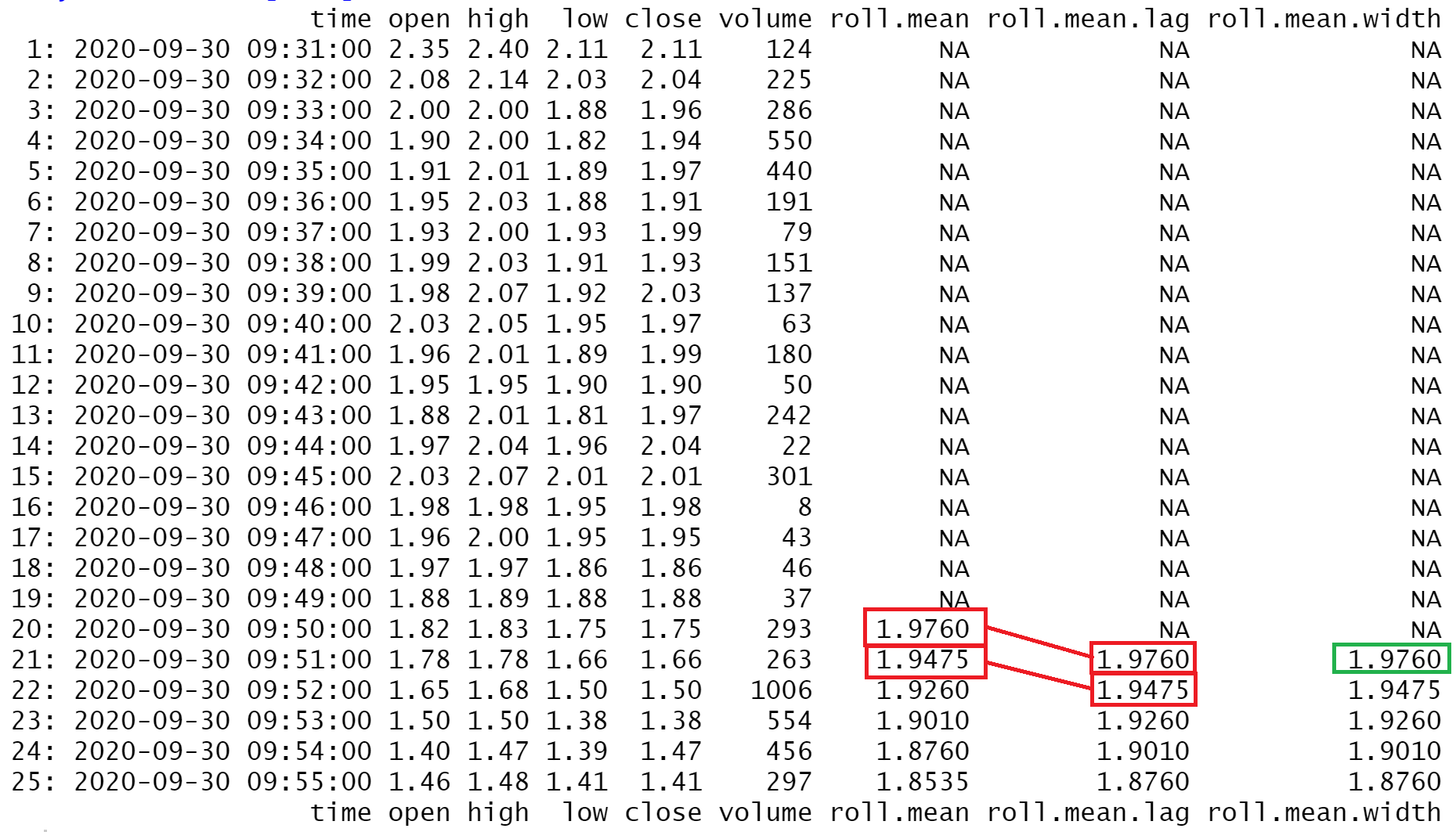
Whatever solution you choose, make sure your data lines up!!