Stock Measured Moves, Implied Volatility and Historical Volatility: A New Metric for Measuring Volatility
TOC
- [Why Are IV and HV So Complicated?](#why-are-iv-and-hv-so-complicated)
- [What We Think We Know We Need to Know (What?)](#what-we-think-we-know-we-need-to-know-what)
- [An Example](#an-example)
- [Another Example](#another-example)
- [A New Measurement](#a-new-measurement)
	- [R Code Overview](#r-code-overview)
- [Example of Measured Move Table](#example-of-measured-move-table)
- [How does Measured Moves compare to HV or IV?](#how-does-measured-moves-compare-to-hv-or-iv)
- [Conclusion](#conclusion)
- [Next steps:](#next-steps)
- [Notes and Research](#notes-and-research)
Why Are IV and HV So Complicated?
Implied Volatility (“IV”) and Historical Volatility (“HV”) have never felt “right” to me.
That is, I can’t wrap my head around the definition: “the implied volatility (IV) of an option contract is that value of the volatility of the underlying instrument which, when input in an option pricing model (such as Black–Scholes), will return a theoretical value equal to the current market price of said option.” Wikipedia - Implied Volatility.
This one from Investopedia is a little clearer: “Implied volatility is the market’s forecast of a likely movement in a security’s price. It is a metric used by investors to estimate future fluctuations (volatility) of a security’s price based on certain predictive factors.”
So then IV is predictive, right? “Implied volatility (IV) refers to a stock’s anticipated volatility of the stock in the future, without regard for direction.” Investing in Options: A Beginner’s Guide.
What about the past stock change? That is covered by historical volatility (“HV”): “In finance, volatility (usually denoted by σ) is the degree of variation of a trading price series over time, usually measured by the standard deviation of logarithmic returns. Historic volatility measures a time series of past market prices. Implied volatility looks forward in time, being derived from the market price of a market-traded derivative (in particular, an option).”
Or this definition from The Options Playbook simplifies HV as: “how much the stock price fluctuated on a day-to-day basis over a one-year period”.
So IV is the predicted price change (plus or minus) during a defined period. HV is the actual price change (plus or minus) during a defined period.
Do the definitions stop there? No! The IV (and the HV) usually gets “annualized” and then that starts all kind of fun. The number you most often see when IV or HV is referred to in finance is the annualized standard deviation of: (1) the underlying instrument’s returns over the past year (or possibly the prior 12 months) for HV; and, (2) the next or future year (12 months?) returns for IV (but see more on this below all you Black-Scholes fans). Then if you want to translate the annualized IV or HV to daily IV or HV you can divide by the square root of 252. Or simply divide either by 16.
So does this mean if Stock A has an HV of 20%, you can assume the stock will go up about 1.25% (20% divided by 16) the next day? No again! Recall that HV and IV are directionally agnostic (they don’t measure whether the stock moves up or down just that it moves a certain percentage on average). And remember IV is generally derived from a statistical model like Black-Scholes or the Binomial method that generally assume a normal or lognormal distribution of returns. Assuming a normal distribution, IV represents a given probability that the stock will move up or down by a certain amount. Applying these models, Stock A with an annual IV of 20% then has a 68.27% (one standard deviation of the mean) of being up or down 20% by the end of the year.
The other fly in the ointment is that HV and IV usually don’t factor in “the expected mean return over the period in which you wish to calculate probability”. This presents an interesting challenge for the technician; without knowing a mean value of the stock’s return, you are unable to calculate the probability of a future value of the underlying.
To illustrate the importance of this omission, consider this example problem: Given that the standard deviation (i.e., “volatility”) of the height of an adult American male is about 3”, what is the probability that the next adult American male you pass on the street is taller than 6’ 0”? Clearly, there is insufficient information to answer this; what’s missing is the average (or mean) height of an adult American male. Link
In other words, if you don’t know the mean, there is no way to find the probability of a specific return occurring. Most calculations get over this limitation by using a defined look-back window to determine a mean value or just using the most recent close. Even applying the HV of 20% to Stock A appropriately, you then must decide whether to use the most recent value of Stock A (which may or may not be close to the mean) or use the mean value of Stock A’s price over some defined window (and the mean may be “far” away from the most recent closing price).
Based on this new information, I need to amend the definition. IV is the predicted price change (plus or minus) during a defined period using a set look-back period to calculate the mean and standard deviation which determines the probability of an expected return based on a normal distribution. HV is the same definition but replace predicted with actual price change.
Yikes. That’s a lot to take in, right? And that doesn’t even get into terms like:
- IV percentile which “calculates the percentage of days in the past 52-weeks in which the IV was lower than the current level”,
- IV rank that “gauges the current level of IV relative to the IV range over the past 52-weeks”,
- IV skewness “Volatility skewness, or just skew, describes the difference between observed implied volatility with in-the-money, out-of-the-money, and at-the-money options with the same expiry date and underlying” Source), or
- other big words I don’t want to define.
What We Think We Know We Need to Know (What?)
What do you need to know about a stock when you are selling an option? To borrow a few cliché analogies, shorting an option is like acting as a casino taking the other side of a bet or an insurance company assuming the risk of loss for an auto, a house or even a life.
A casino knows the odds that, over a large enough number of bets, they will profit by a certain amount. This “house edge” is enviable from an investor’s perspective because it can be proved mathematically and it is independent of any historical data. For example:
In American Roulette, there are two zeroes and 36 non-zero numbers (18 red and 18 black). If a player bets $1 on red, his chance of winning $1 is therefore 18/38 and his chance of losing $1 (or winning -$1) is 20/38.
The player’s expected value, EV = (18/38 x 1) + (20/38 x -1) = 18/38 - 20/38 = -2/38 = -5.26%. Therefore, the house edge is 5.26%. After 10 rounds, play $1 per round, the average house profit will be 10 x $1 x 5.26% = $0.53. Of course, it is not possible for the casino to win exactly 53 cents; this figure is the average casino profit from each player if it had millions of players each betting 10 rounds at $1 per round.
Casino’s don’t care what happened over the prior 20 spins of the roulette wheel; variance doesn’t matter since they have a big enough pot of cash. They know that in the long run, they will end up ahead.
Insurance companies operate in a similar manner but instead of proving the “house edge” mathematically, they prove it based on the historical experience rating of whatever it is they are insuring. This is referred to as underwriting the financial risk they are assuming through the process of actuarial science. Casinos and insurance companies also share some of the same financial metrics when assessing the strength of different stocks.
Option sellers want to be the house or the insurance company. They want to know the historical odds that the underlying instrument will move against or for their position. Ideally, these odds can be proved mathematically (like a casino at the roulette wheel) or through repeating historical events that are very probable to happen again (like an insurance company underwriting life insurance claims based on mortality tables). This is simplistic for a couple of reasons discussed below, but it’s a start. But since most individual option sellers don’t have the capital that a casino or an insurance company has to withstand the variance, they need to tilt the scales more in their favor. Can you improve on traditional measures of IV and HV? That’s what the rest of this post seeks to understand.
An Example
Assume for a second that you are given daily stock data going back 250 trading days. You know nothing about the stock or it’s fundamentals. You only have the price data.
What’s the HV? Black-Scholes style we want the annualized standard deviation of the log returns of the adjusted close.
data.past <- all.sym[1:250,]

ret <- log(lag(data.past$adjusted.close, n = 1, default = 0)) - log(data.past$adjusted.close)

vol <- sd(ret[2:250]) * sqrt(250)
last.close <- data.past[250,]$adjusted.close

vol
last.close

#> vol
#[1] .1709717

#> last.close
#[1] 198.3989
Annualized percent volatility is then 17.7% and the stock last closed at 198.39.
After you calculate the HV, you are asked to determine what the price will be after the next 250 days.
One option is to give a range of probabilities based on a normal distribution of returns. Assuming the last.close() is the mean and the vol() is the standard deviation, we can say with about 95% confidence that the final price will be between -1.96 and +1.96 standard deviations of the mean.
option1.upper <- last.close * (1+vol*1.96)

option1.lower <- last.close * (1-vol*1.96)

#> option1.upper
#[1] 264.8833
#> option1.lower
#[1] 131.9145
Option 1 predicts with 95% certainty that the stock will be between 131 and 264.
The second option is to look at the average price over the last year and calculate our 2-standard deviation range from there.
option2.avg <- mean(data.past$adjusted.close, na.rm = T)

#> option2.avg
#[1] 184.1292

option2.upper <- option2.avg * (1+vol*1.96)

option2.lower <- option2.avg * (1-vol*1.96)

#> option2.upper
#[1] 245.8317
#> option2.lower
#[1] 122.4267
Option 2 gives a slightly smaller window for the 95% confidence interval. Using this method predicts the stock will close between 122 and 245.
There is one more method to consider. Option 3 is to examine the average of a given look back period from each period and then take the average of those averages (what?). For example, find the average price and average volatility over the prior 20 days from the close of each daily period. At the end of 250 days, you average each of these results and use those values to calculate the 95% confidence interval.
option3.avg <- sma(data.past$adjusted.close, 20)

# - Note that roll_sd returns the point value of the standard deviation - it is transformed to an annualized percentage by dividing by the prior adjusted close and multiplying that times the square root of 250

option3.vol <- roll_sd(data.past$adjusted.close, 20)/lag(data.past$adjusted.close, n = 1)*sqrt(250)

option3.avg.total <- mean(option3.avg, na.rm = T)
option3.vol.total <- mean(option3.vol, na.rm = T)

option3.upper <- option3.avg.total * (1+option3.vol.total*1.96)

option3.lower <- option3.avg.total * (1-option3.vol.total*1.96)

option3.upper
option3.lower

#> option3.upper
#[1] 280.4202
#> option3.lower
#[1] 86.52874
Option 3 predicts a volatile year with upper and lower returns of 280 and 86, respectively. (Note: you can re-do this calculation with a 50-day look back window and the range becomes even bigger - 38 lower and 328 upper!)
| Lower | Upper | Difference | |
|---|---|---|---|
| Option 1 | 131 | 264 | 133 |
| Option 2 | 122.4 | 245.8 | 123.4 |
| Option 3 | 86.5 | 280.4 | 193.9 |
After you make the handy-dandy table, you are magically given the next (future) 250 days of the stock price and told to compare the actual results with what you predicted.
data.future <- all.sym[251:500,]

last(data.future$adjusted.close)

summary(data.future$adjusted.close)

#> summary(data.future$adjusted.close)
#   Min. 1st Qu.  Median    Mean 3rd Qu.
#  192.3   200.0   210.6   211.4   221.0
#   Max.
#  231.2
Using the handy last() and summary() functions, we find out that the price a year from now is 231.2 (which coincidentally is also the high). All 3 options you created did the job; price fell within the window each formula predicted. You won!
But are the calculated ranges given by normal distribution useful information? We could have just as easily said that price would end up between 0 and 1,000,000 and been just as “right” about our prediction as any of the 3 options. Black-Scholes and the rest counter that the normal distribution component is an assumption based on many different possible cumulative returns. In some alternate universe, the price could have just as easily been 264 at the end of the year. That’s true and that helps casinos and insurance companies make decisions when dealing with a large number of bettors or insureds. Normal distribution becomes less enticing when selling an option on a single underlying, with a single expiration date and a single strike price. There are no re-dos in option selling, nor are there alternate universes. There is only a stock that moves one way or the other and a potential margin call if one of those universes ends up askew.
Another Example
Assume you are asked to create an American style ATM call and put option (a strangle) to sell on our “mystery” stock expiring in 250 trading days. What information other than the days to expiration would you have to know to determine the price of the option? The current price of the underlying and the expected movement (volatility) would be the bare minimum. You could use this information to crudely price this option based on HV.
Greater minds than me have calculated this before me. The call and put price can be estimated using several different formulas.
This one which is directly from here and mentioned in the answer to this question:
call_price = put_price = 0.4Svolsqrt(T) = 0.021Svolsqrt(D)
price = in dollars S = underlying spot price vol = volatility in percent T = time in years D = time in days
ATM Strangle = 1/2000 * Current Price * Annualized Volatility * Square Root of Days to Expiration
Or use an online calculator.
Plugging the two formulas into R, you get about the same result for the ATM strangle:
198*.4*.177*sqrt(250/252)*2

1/2000*198*17.7*sqrt(250)

#> 198*.4*.177*sqrt(250/252)*2
#[1] 27.92532
#>
#> 1/2000*198*17.7*sqrt(250)
#[1] 27.7063
This is somewhat inline with our results above (except it assumes a one-standard deviation move).
R can easily calculate the Black-Scholes formula to give us the put and call prices for our ATM strangle:
Call <- function(S, K, r, T, sigma) {
  d1  <-  (log(S/K) + (r + sigma^2/2)*T) / (sigma*sqrt(T))
  d2  <-  d1 - sigma*sqrt(T)
  S * pnorm(d1)  - K*exp(-r*T)*pnorm(d2)
}

Put <- function(S, K, r, T, sigma) {
  d1  <-  (log(S/K) + (r + sigma^2/2)*T) / (sigma*sqrt(T))
  d2  <-  d1 - sigma*sqrt(T)
  -S * pnorm(-d1) + K*exp(-r*T)*pnorm(-d2)
}
Where the variables are defined as follows:
| Variable | Description | Example |
|---|---|---|
| S | Spot Price | 198 |
| K | Strike Price | 198 |
| r | risk-free interest rate | 0 |
| T | Time to Maturity | 1 => 252/252 trading days |
| sigma | Implied annual volatility | 17.7% |
Call(198,198,0,1,.177)
#>[1] 13.9631

Put(198,198,0,1,.177)
#>[1] 13.9631

13.9631 + 13.9631
#>[1] 27.9262
Man! Those rules of thumb save a lot of typing!
So you feel good selling the option at 27.9 based on the known variables. You are content to bank your money and hang out for a year to see what happens.
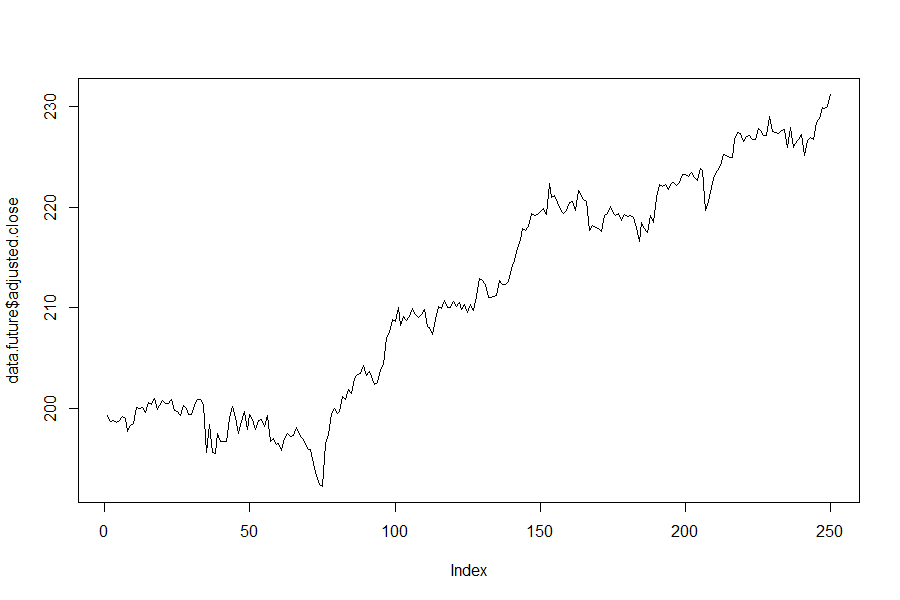
If you knew price would do this, would you change the price of the strangle? Probably not (BTW this is the actual path of the underlying stock):
What about these two graphs - same starting and ending points, same minimum and maximum price based on a 2 SD move but now there is a spike or drop in the price for about 100 days?
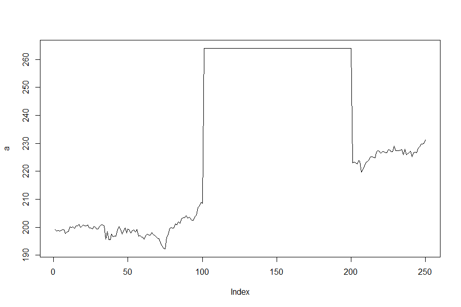
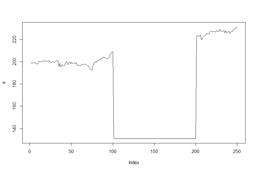
Yikes, well that’s a horse of a different color! (And before anyone points out that the stats would change if the stock moved up to 264 or down to 131 for 100 days, ie, the historical mean and standard deviation would change, I get it but stick with me for the sake of argument). Even though each stock price ended up the same the path to get there was much different. It’s like the difference in going from your house to the store by taking a city bus versus riding the bus for a few minutes, getting on a space shuttle and rocketing to the moon and back, and then catching the bus at a later stop to finish your trip. Sure you get the same bag of Cheetohs at the store at the end of both scenarios, but the second path is one hell of a better ride.
This (terrible) analogy illustrates another issue with using normal or lognormal distribution to measure stock path movement to price options. Normal measurements ignore time in the sense that there is no connection between the historical price data and the historical time data. At first glance, it appears that price is not accounted for properly, but that’s not defining the problem correctly. You (hopefully) gasped at the second two graphs above because price went up so high or low and then stayed there for a long time before returning to earth. Normal distribution doesn’t factor in whether the stock goes from 198 to 192 and stays there for 11 months before closing at 231 in the last 10 days. Or if price bounces up and down (range-bound) for an extended period of time. Normal distribution doesn’t care about the time it takes a stock to go to one place or the other; only that the price could reach one price or another. And that’s a terrible problem to have when the stock shoots for the moon suddenly.
A New Measurement
Based on the above, an ideal measurement to price an option based on an underlying instrument’s future movement would: (1) be shown mathematically through probability based on the known historical data at hand, (2) not be subject to a pre-defined look back window (which could introduce a level of unconscious bias), (3) be based on the maximum or minimum value of the actual expiration date of the option you are selling, and (4) perhaps most importantly, factor in when it is likely that a price may move one way or the other.
R Code Overview
The R code uses daily stock data because of its wide availability. If you have an IQFeed account, you can run it for time periods less than daily by changing the increment.period() to tick, 1min, 5min, 10min, 15min, 30min, hour, day, week, month etc.
Second, each function will use a “rolling approach” - all data points are considered, rather than just specific look back periods. For example, assume we are evaluating 100 days of daily AAPL data. The functions that measure how far positive and how far negative price goes will be evaluated starting from day 1 to day 2, day 1, to day 3 etc. all the way up to day 1 to day 100. It then cycles to day 2 and evaluates from day 2 to day 3 and on. The look forward periods are set but will be dynamic; this means that the code will return multiple look forward periods to match a given options expiration.
Continuing the AAPL example, this means that for each of the 100 days, it will look forward from 1 to x number of days. On day 1, it will look forward to day 2, then day 3 etc. On day 2, to day 3 then day 4 and so on. The code really only has 2 dynamic variables - the ticker symbols and the maximum number of days to look forward from each data point. What it measures is the total number of times price moved from one point to the next over a defined time series.
Example of Measured Move Table
Here is a snippet of a chart showing measured moves:

You can read the table as follows:
- Each table represents one individual stock.
- The first column is the percent plus which is a defined percentage move to a higher price or percent minus which is a defined percentage move to a lower price. Each percentage plus or minus is measured from every single historical price period.
- The first row represents the number of periods that each measurement “looked-forward.”
- Each data point is the mean percentage of times the given stock moved up or down during the given look back period.
- For example, the “0.62” highlighted in the red box means that on average, the stock CMS moved down at least 1% over a 10-day period for the time period indicated above the table.
How does Measured Moves compare to HV or IV?
So now that we have this tool, how do we use it? And how does it compare to HV or IV?
First, we need to find the historical volatility for each stock. This requires a few assumptions. I have to choose a “look-back” window for the each ticker to find the average standard deviation over the given time period. In this instance, I will use the same periods set forth in the limit.period.2 variable (which are 5, 10, 20, 50 and 100). Once I have all of these “rolling windows”, I have to average all of the values to get a single number for the standard deviation of the returns for each stock (based on each look-back window).
Second, I can use this value to determine the probability, based on the normal distribution, that a stock will be less than or greater than a given percentage. I have created a function called fn.probability() that calculates this probability. The strike input can be calculated by taking a percent.plus or a percent.minus increment and adding it to 1. For example, if the stock’s current.price is 1, then a 1% move would take it to 1.01. Further, the DTE variable is also matched up with each limit.period.2 value.
# - using a normal distribution, returns the probability that the stock will be below (when strike is greater than price) or above (when strike is less than price) the strike at expiration
fn.probability <- function(strike, current.price, ann.vol, DTE){
  calc.sd <- ann.vol * sqrt(DTE/365) * current.price
  a <- pnorm(strike, current.price, calc.sd)
  b <- ifelse(strike >= current.price, a, 1-a)
  return(b)
}

# Where each is:
# strike        <-    the strike price of the put or call option ($)
# current.price <-    the current price of the underlying stock ($)
# ann.vol       <-    the annualized volatility - this can be IV or HV (%)
# DTE           <-    the days to expiration of the put or call option
Finally, once I have solved for the hypothetical normal distribution-based probability that a given stock will exceed a given percentage over a specified time, I can compare that to the actual stock measured move to see how “accurate” the normal distribution is.

Based on the last 100 days of data and a 1% percent.plus move, the predicted normal distribution for the stocks listed above is between 27% to 43%. For example, I calculated SPY’s average volatility over 5 days, and then used the fn.probability() to determine the normal distribution. This predicted that the stock would move by 1% approximately 27% of the time over 5 days. I then compared this to the measured move (ie, the actual percent of the time the stock moved 1% over the prior 100 days) and found that SPY increased by at least a full percentage point 44% of the time. This results in a diff (calculated as the actual minus the predicted) of 17%. In other words, SPY will move +1% about 37% more of the time than what the normal distribution predicts.
Does this mean that actual options are priced incorrectly? No, because options use IV, or what the collective market believes is going to happen rather than the HV I used to create the Measured Move table. The discrepancy noted above for SPY increasing 1% (44% Measured Move vs 27% Normal Distribution) is because the normal distribution is based on the average of all HV which were calculated over a rolling window of 5 trading days. As of this writing, SPY sits at 384.4, meaning a 1% move is approximately 388. A call with a strike price of 388 with 5 DTE costs 2.88 (according to eTrade), meaning it has an annualized IV of 20.84%.
The R function Call() noted above agrees with this valuation, pricing the option at 2.89.
> Call(384.4,388,0,5/252,.2058)
#[1] 2.895108
Plugging the variables to solve for the probability shows:
> fn.probability(388,384.4,.2048,5)
[1] 0.6519929
Thus, based on the above:
- the market is implying that SPY will move 1% about 65% of the time over 5 days (IV);
- SPY has historically moved 1% about 44% of the time over 5 days (Measured Move); and,
- based on the average HV, the normal probability distribution predicts SPY to increase 1% about 27% of the time (Predicted Normal Distribution).
Ideally, if you are selling options, you want to find those that have the biggest difference between the Predicted Normal Distribution (based on the Measured Move) compared with the IV offered by the market.
Conclusion
IV and HV are readily accepted measures when determining option prices. However, they can be overly complicated for some people (like myself). Measured Moves, and by extension the predicted normal distribution, are somewhat simpler way to visualize HV and then compare that to what the market is offering through IV.
Next steps:
- Utilize high and low in the Measured Moves. Remember that all of the data herein uses closing prices; using high and low values will alter the results. Future iterations of this model will implement high values for
percent.plusand low values forpercent.minus. - Implement “OR” and “BOTH (AND)”. Since the underlying price moves both up and down before the close, future code should implement: (1) “OR” measures that show the percent of the time that the stock moves past either the
percent.plusor thepercent.minus, and (2) “BOTH (AND)” measures that illustrate the percent of the time the stock moves past both thepercent.plusAND thepercent.minus. - Convert the Measured Move Metric to Expectancy. Assuming that the HV continues into the future, and based on the current IV, what is the maximum loss a system can withstand before having a negative expectancy. This should help with setting stops etc.
- Filter Current Options for Opportunity. The last improvement would be to identify options that have the largest historical difference between the normal predicted distribution and the option’s current IV. This, combined with the expectancy calculation, would be a good basis for identifying opportunities.
Thanks for reading!
Notes and Research
-
[Betting Odds Calculator & Converter The Action Network](https://www.actionnetwork.com/betting-calculators/betting-odds-calculator) -
[The Importance Of Differentiating Between Historic And Implied Probability Seeking Alpha](https://seekingalpha.com/article/397431-the-importance-of-differentiating-between-historic-and-implied-probability) -
[Investing In A Paranormal Market - February Update Seeking Alpha](https://seekingalpha.com/article/380531-investing-in-a-paranormal-market-february-update) - I Volatility - Options Calculator
- IVolatility.com - Compare Packages
- Stock Options Analysis and Trading Tools on I Volatility.com
- IVolatility.com -
-
[Are Market Implied Probabilities Useful? Flirting with Models](https://blog.thinknewfound.com/2017/11/market-implied-probabilities-useful/) - Implied Volatility: Spotting High Vol and Aligning Yo…- Ticker Tape
- Credit Spreads vs. Debit Spreads: Let Volatility Decide- Ticker Tape
-
[Heads I Win, Tails I Hedge Flirting with Models](https://blog.thinknewfound.com/2020/07/heads-i-win-tails-i-hedge/) -
[14.1 - Probability Density Functions STAT 414](https://online.stat.psu.edu/stat414/lesson/14/14.1) -
[Options Volatility Implied Volatility in Options - The Options Playbook](https://www.optionsplaybook.com/options-introduction/what-is-volatility/) -
[Investing in Options: A Beginner’s Guide Part 3 Understanding Volatility Ally](https://www.ally.com/do-it-right/investing/investing-in-options-a-beginners-guide-part-3-understanding-volatility/) - Implied Volatility – IV Definition
- Converting Implied Volatility to Expected Daily Move - Macroption
- Volatility Rule of 16 - Macroption
- Implied Volatility Calculator - Macroption
- ch5.pdf
- Resolution : Choosing the Appropriate Commodity Option Pricing Model
- Volatility (finance) - Wikipedia.)
- Volatility (finance) - Wikipedia
- https://www.tastytrade.com/shows/options-jive/episodes/difference-between-iv-rank-and-iv-percentile-02-19-2016
-
[Volatility Skewness IV Skew In Options](https://epsilonoptions.com/volatility-skewness/#:~:text=Volatility%20skewness%2C%20or%20just%20skew,same%20expiry%20date%20and%20underlying.) - Gambling mathematics - Wikipedia
- probability - Does variance do any good to gambling game makers? - Mathematics Stack Exchange
-
[Insurance Is Gambling, Seriously Seeking Alpha](https://seekingalpha.com/article/4080260-insurance-is-gambling-seriously) - Actuarial science - Wikipedia
- Ruin theory - Wikipedia
- r - How to calculate stock volatility in %? - Cross Validated
- Chapter-6-R.pdf
-
[Are Stock Returns Normally Distributed? by Tony Yiu Towards Data Science](https://towardsdatascience.com/are-stock-returns-normally-distributed-e0388d71267e) -
[What In The World Are QQ Plots?. Understanding What QQ Plots Do And How… by Tony Yiu Towards Data Science](https://towardsdatascience.com/what-in-the-world-are-qq-plots-20d0e41dece1) - Markdown Tables generator - TablesGenerator.com
- Law of large numbers - Wikipedia
-
[Straddle Approximation Formula Brilliant Math & Science Wiki](https://brilliant.org/wiki/straddle-approximation-formula/) - options - What are some useful approximations to the Black-Scholes formula? - Quantitative Finance Stack Exchange
- Espen Haug
- Rule of thumb for option prices cheatsheet : options
- Short Guts
- Option Price Calculator
-
[Straddle Approximation Formula Brilliant Math & Science Wiki](https://brilliant.org/wiki/straddle-approximation-formula/) - options - What are some useful approximations to the Black-Scholes formula? - Quantitative Finance Stack Exchange
- Black-Scholes option pricing
- R name colnames and rownames in list of data.frames with lapply - Stack Overflow
- Plot multiple lines (data series) each with unique color in R - Stack Overflow
-
[renv: Project Environments for R RStudio Blog](https://blog.rstudio.com/2019/11/06/renv-project-environments-for-r/) - R Length of vector without NA’s
- r - Reduce size of legend area in barplot - Stack Overflow
- Add a legend to a base R chart – the R Graph Gallery
- Tables · Bootstrap
- r - Concatenate a vector of strings/character - Stack Overflow
- Volatility Trading - Converting Annual to Daily Volatility - Raging Bull
-
[Simple Trick to Convert Volatility Volatility Futures & Options](http://onlyvix.blogspot.com/2010/08/simple-trick-to-convert-volatility.html) -
[Option Probability Curve Option Alpha](https://optionalpha.com/members/video-tutorials/pricing-volatility/option-probability-curve) - Option Strangles: An Analysis of Selling Equity Insurance
-
[What To Watch Out For In High-Probability Strategies Seeking Alpha](https://seekingalpha.com/article/4356459-what-to-watch-out-for-in-high-probability-strategies) -
[Selling Straddles Profit & Loss Frequencies STUDY projectoption](https://www.projectoption.com/selling-straddles-profit-loss-frequency/) - Combinations and permutations in R - Dave Tang’s blog
-
[Learning R: Permutations and Combinations with base R R-bloggers](https://www.r-bloggers.com/2019/06/learning-r-permutations-and-combinations-with-base-r/) - if statement - Double match in r - Stack Overflow
- values exist in data.table in multiple columns R - Stack Overflow
-
[AI for algorithmic trading: rethinking bars, labeling, and stationarity by Alexandr Honchar Towards Data Science](https://towardsdatascience.com/ai-for-algorithmic-trading-rethinking-bars-labeling-and-stationarity-90a7b626f3e1) - data.table - How to calculate the mean of the top 10% in R - Stack Overflow
- How to convert volatility from annual to daily, weekly or monthly? – Banking School
- Loops in R – Programming with R