Measuring Momentum vs Mean Reversion Trading Systems for 2015-2020
Overview/Summary
This post examines momentum and mean reversion systems and whether S&P500 stocks exhibited behavior supporting one or the other theories.
TOC
- Introduction
- Part 1: Building the Mean Reversion and Momentum Systems
- R-Code for Individual Stock Analysis
- An Example Multi-Variate Logistical Regression System
- Notes and Research
Link to all R-Code Link to this Post’s R-Code on Github
Introduction
jump back to top Other than a few exceptions, most trading systems can be divided into two categories: (1) mean reversion systems, and (2) momentum systems. “Mean reversion, or reversion to the mean, is a theory used in finance that suggests that asset price volatility and historical returns eventually will revert to the long-run mean or average level of the entire dataset.” Investopedia Definition of Mean Reversion. Conversely, “[m]omentum investing is a trading strategy in which investors buy securities that are rising and sell them when they look to have peaked.” Introduction to Momentum Investing.
Both mean reverting and momentum trading systems are opposite sides of the same coin. They seek to answer the question: if a stock has increased or decreased for X number of periods, is it more likely to return to the mean or continue to increase or decrease over the next Y number of periods? How you define X & Y number of periods, measure the increase or decrease of the stock and measure the mean can all be parameters built into the trading system.
One popular mean reversion strategy is to buy when price is 2 or more standard deviations (“SD”) below the simple moving average (“SMA”) and sell short when price is 2 or more standard deviations above the SMA. The converse then could be true for a momentum system - you would sell short if price is below 2 SD and go long when price is above 2 SD.
In the first part of the code, I try to answer the question on a broad basis by examining the performance of a system that entered at every point along the time series that satisfied the mean reverting system paramater.
The second part of the code attempts to measure the returns of each instrument over varying look-forward periods after price crosses over or under +/- 2 SD.
The final part of the code examines the performance of a simple multivariate linear regression system using the indicators and measures utilized in the first two parts.
Part 1: Building the Mean Reversion and Momentum Systems
jump back to top From a coding standpoint, it is easier to start with a mean reversion system than a momentum system. Mean reversion posits that periods of the price decreasing are followed by periods of price increasing and vice versa. It seeks to see if it is more probable that price will return to an average price after a period of under or over performance.
First, you I have to quantify what it means for price to underperform (referred to as being oversold or “OS”) or overperform (overbought or “OB”). One measure is to look at the historical volatility of the stock in relationship to a moving average. Since historical volatility is the standard deviation of price over a given number of days, using a z-score in this instance makes sense. Z-scores measure how far below or above price is from a moving average. For example, a z-score of -2 means that price is 2 SD below the SMA. See Mean Reversion: Simple Trading Strategies Part 1. As noted in the introduction, our mean reversion strategy goes long when the z-score is -2 and goes short when the z-score is +2.
R-Code for Z-Score
jump back to top After setting the parameters and downloading the stock data for the S&P 500 see full R code here the indicators can be defined as follows:
#- solve for simple moving average of close
df.sma <- lapply(ind.sym, function(x)(sma(x$close,p.sma.period)))

#- solve for standard deviation of close
df.sd <- lapply(ind.sym, function(x)(roll_sd(x$close,p.sd.period)))

# - number of standard deviations that price above or below the SMA
df.zscore <- mapply(function(x,y,z)((x-y$close)/z),df.sma,ind.sym,df.sd,SIMPLIFY=F)

# - location/index where z-score exceeded lower and upper z-score bounds
df.lower.zscore <- lapply(df.zscore, function(x)(which(x <= p.lower.zscore)))
df.upper.zscore <- lapply(df.zscore, function(x)(which(x >= p.upper.zscore)))
There are two paramaters to adjust or change as needed based on your own assumptions: p.sma.period() and p.sd.period(). Since I am utilizing a dynamic (i.e., continuous and non-discrete) time series, I have to utilize rolling windows of look-back periods to calculate the SMA and the SD. You can modify these as needed to suite your trading timeframe.
R-Code for the Look-Forward and Look-Back Analysis
jump back to top The key point for this code is that we are examining every point along the time series, regardless of whether it is greater than or less than the upper or lower z-score. From each point, the code measures the return over multiple look-forward and look-back periods. Take a look at the example data frame below:

Each column beginning with “lf” looks from one period after the current period until the periods noted. So the first row in column lf.20 measures the cumulative return from the second row to the twenty-first row. The look-back or “lb” rows measure from one period prior to the given period back to the number of periods indicated - lb.5 measures the cumulative return from 6 periods before row 1 to the period just before row 1. The reasoning why return is offset one period comes from the fact that the signal and the entry cannot occur on the same period (or bar if thinking in graphical terms). For example, if the z-score is below the threshold in row 5, entry could not occur until row 6.
The remainder of the code adds the look-back and look-forward columns and returns the locations where the z-score was less than the lower level indicated (here below -2 SD based on a 20 period SMA and SD window) and where the z-score was greater than the upper level (+2 SD).
df.all.sym <-
  lapply(ind.sym, #9 columns
    function(x)(
      x %>%
        mutate(
          lf.1 = lead(close,n=2)/lead(close,n=1)-1,     #10
          lf.2 = lead(close,n=3)/lead(close,n=1)-1,     #11
          lf.3 = lead(close,n=4)/lead(close,n=1)-1,     #12
          lf.4 = lead(close,n=5)/lead(close,n=1)-1,     #13
          lf.5 = lead(close,n=6)/lead(close,n=1)-1,     #14
          lf.10 = lead(close,n=11)/lead(close,n=1)-1,   #15
          lf.20 = lead(close,n=21)/lead(close,n=1)-1,   #16
          lf.50 = lead(close,n=51)/lead(close,n=1)-1,   #17
          lb.1 = lag(close,n=2)/lag(close,n=1)-1,       #18
          lb.2 = lag(close,n=3)/lag(close,n=1)-1,       #19
          lb.3 = lag(close,n=4)/lag(close,n=1)-1,       #20
          lb.4 = lag(close,n=5)/lag(close,n=1)-1,       #21
          lb.5 = lag(close,n=6)/lag(close,n=1)-1,       #22
          lb.10 = lag(close,n=11)/lag(close,n=1)-1,     #23
          lb.20 = lag(close,n=21)/lag(close,n=1)-1,     #24
          lb.50 = lag(close,n=51)/lag(close,n=1)-1,     #25
          my.sma = sma(close,p.sma.period),             #26
          my.sd = roll_sd(close,p.sd.period),           #27
          z.score = (my.sma-close)/my.sd                #28
        )
      )
    )

df.all.sym.bind <- rbindlist(df.all.sym)

# - return all the locations of df.all.sym where z-score was less than lower level
df.lower.forward <-
  lapply(seq_along(ticker),
    function(x)(
      df.all.sym[[x]][df.lower.zscore[[x]],]
    )
  )
all.lower <- rbindlist(df.lower.forward)

# - return all the locations of df.all.sym where z-score was greater than upper level
df.upper.forward <-
  lapply(seq_along(ticker),
    function(x)(
      df.all.sym[[x]][df.upper.zscore[[x]],]
    )
  )
all.upper <- rbindlist(df.upper.forward)
Z-Score System Analysis for All S&P500 Stocks from 2015-2020
jump back to top
Using the above, I looked at data for all S&P500 stocks for 2015-2020 (year by year) and using individual look-forward periods of c(1,2,3,4,5,10,20,50) days I calculated the average cumulative returns when price (open) was less than -2 SD or more than +2 SD and compared that to all cumulative returns regardless of the price relationship to the z-score. I used SD and SMA windows of 20 periods.
For each table below, the first column contains the look-forward period, column two is the average cumulative return following price dropping below the lower z-score threshold, and column three is the same average return calculation for the upper z-score threshold. The last column is the average for all returns, regardless of the price’s relationship to the z-score. For example, the Table: 2020 Returns, looking at the second to last row for lf.20, when price closed lower than the lower z-score, the average cumulative return over the next 20 days was -0.17%. When price closed greater than the upper z-score threshold, the average cumulative return was -1.63% over the next 20 days. Compare both of these for all average cumulative returns for all z-scores of 1.59%. The tables for years 2015-2020 are given below.
Table: 2020 Returns (%)
| look forward period | lower z-score | upper z-score | all |
|---|---|---|---|
| lf.1 | -0.26608 | -1.30345 | 0.08968 |
| lf.2 | -0.64965 | -1.20974 | 0.16485 |
| lf.3 | -0.64498 | -1.02758 | 0.25304 |
| lf.4 | -0.50871 | -1.69287 | 0.33586 |
| lf.5 | -0.40968 | -1.81274 | 0.40628 |
| lf.10 | -0.27123 | -4.04107 | 0.75864 |
| lf.20 | -0.17712 | -1.63468 | 1.59696 |
| lf.50 | 3.46289 | 4.71229 | 4.03506 |
Table: 2019 Returns (%)
| look forward period | lower z-score | upper z-score | all |
|---|---|---|---|
| lf.1 | 0.06147 | 0.17841 | 0.12032 |
| lf.2 | 0.10460 | 0.34758 | 0.22701 |
| lf.3 | 0.12210 | 0.36068 | 0.33181 |
| lf.4 | 0.16603 | 0.49065 | 0.43360 |
| lf.5 | 0.20887 | 0.63016 | 0.53293 |
| lf.10 | 0.37685 | 0.71543 | 1.01239 |
| lf.20 | 0.18879 | 1.89274 | 1.83416 |
| lf.50 | 2.52901 | 4.24761 | 3.65635 |
Table: 2018 Returns (%)
| look forward period | lower z-score | upper z-score | all |
|---|---|---|---|
| lf.1 | -0.13054 | -0.02425 | -0.02633 |
| lf.2 | -0.21027 | -0.07012 | -0.05762 |
| lf.3 | -0.35198 | 0.13565 | -0.09118 |
| lf.4 | -0.43232 | 0.20123 | -0.12890 |
| lf.5 | -0.47084 | 0.17033 | -0.18650 |
| lf.10 | -0.85711 | -0.00246 | -0.37794 |
| lf.20 | -0.54546 | 1.19745 | -0.57700 |
| lf.50 | -0.20564 | -1.19750 | -0.53248 |
Table: 2017 Returns (%)
| look forward period | lower z-score | upper z-score | all |
|---|---|---|---|
| lf.1 | 0.06376 | 0.05400 | 0.07574 |
| lf.2 | 0.13202 | 0.10598 | 0.15511 |
| lf.3 | 0.20670 | 0.18558 | 0.23293 |
| lf.4 | 0.29513 | 0.23003 | 0.31305 |
| lf.5 | 0.37640 | 0.30515 | 0.39277 |
| lf.10 | 0.64002 | 0.53423 | 0.79202 |
| lf.20 | 1.14013 | 1.52707 | 1.56715 |
| lf.50 | 3.29172 | 3.18820 | 3.48967 |
Table: 2016 Returns (%)
| look forward period | lower z-score | upper z-score | all |
|---|---|---|---|
| lf.1 | -0.00008 | 0.31203 | 0.06647 |
| lf.2 | 0.03464 | 0.61222 | 0.14131 |
| lf.3 | 0.02562 | 0.85886 | 0.22555 |
| lf.4 | 0.06912 | 0.94940 | 0.31938 |
| lf.5 | 0.14938 | 1.19007 | 0.41367 |
| lf.10 | 0.53573 | 2.54242 | 0.92398 |
| lf.20 | 1.47979 | 4.00344 | 1.98822 |
| lf.50 | 2.61306 | 6.57660 | 4.65101 |
Table: 2015 Returns (%)
| look forward period | lower z-score | upper z-score | all |
|---|---|---|---|
| lf.1 | -0.00654 | 0.41919 | 0.01696 |
| lf.2 | 0.06961 | 0.78555 | 0.04166 |
| lf.3 | 0.00646 | 1.00356 | 0.06350 |
| lf.4 | -0.02758 | 0.91946 | 0.07415 |
| lf.5 | -0.01443 | 0.91569 | 0.08748 |
| lf.10 | -0.02538 | 1.37739 | 0.14771 |
| lf.20 | 0.06791 | 0.70396 | 0.24964 |
| lf.50 | -0.81918 | 1.66457 | 0.36577 |
Assume that price responds within 5-days when a given z-score threshold is breached. The years can be summarized then as follows:
Table: Summary of 2015-2020 Returns (%) for 5-Period Look-Forward
| year | lower z-score | upper z-score | all |
|---|---|---|---|
| 2015 | -0.01443 | 0.91569 | 0.08748 |
| 2016 | 0.14938 | 1.19007 | 0.41367 |
| 2017 | 0.37640 | 0.30515 | 0.39277 |
| 2018 | -0.47084 | 0.17033 | -0.18650 |
| 2019 | 0.20887 | 0.63016 | 0.53293 |
| 2020 | -0.40968 | -1.81274 | 0.40628 |
To “prove” the mean reversion theory, you would expect that for stocks that open below -2 SD, the return would be GREATER when compared with all stock returns over the same time period. This is because when price reaches some distance below the mean, under a mean reversion theory, it should reverse course and start to increase. The opposite is expected for the upper z-score limit. When price is greater than +2 SD, then you would expect the return to be LESS than the return for all z-scores.
For the lower z-score threshold set at -2 SD, this is not true (on average) for all stocks in the S&P500 from 2015-2020. In fact, the opposite is true; when price breached the lower SD band, it tended to continue in a more negative manner - this is shown in the table by comparing the lower column to the all column and noting that the lower return is less in each year when compared to the return for all stocks. For example, in 2020, stocks that opened lower than -2 SD averaged a cumulative return of -0.40% over the next 5 days versus a 0.40% return for all stocks over the next 5 days.
The upper threshold or “overbought” analysis does not support the mean reversion theory, except in 2017 and 2020. Excluding those two years, price was greater than the all period return. Had price reverted lower to the mean, the upper column would be less than the all column indicating that price reversed course and tended lower after exceeding +2 SD.
Not to say that this gives clear support for the momentum theory (ie, that higher prices follow higher prices and lower prices follow lower prices). However, it does indicate that for S&P500 500 stocks using daily open data for 2015-2020, it is likely that the mean reversion theory was not supported.
Feel free to re-run these tests with different parameters. You can change dates, symbols, SD periods and other items.
R-Code for Individual Stock Analysis
jump back to top
I won’t belabor the review of the code but the next section of R-code examines the individual stocks and their relationship to the z-score. The next “reports” the code generates is based on the decile analysis of the stock returns. It shows the average z-score over a given number of look-forward periods for the lowest 20% and highest 20% of returns (indicated in the code as top.80). In essence, it answers the question “so what was the z-score - or how many standard deviations away from the mean was price - when the best and worst returns occurred?”
Let’s say you have a 5-period window you want to trade a stock; you can only go long, there is no commission or fees and you only have the z-score indicator to determine when to enter. You want to know what z-score you should look at to attain the top returns. The next section of R-code attempts to determine where price was in relationship to the z-score when the top 80% and bottom 20% of returns occurred when measured over 5, 20 and 50 look-forward periods. First, it splits up the returns over each of these periods into deciles. Then it identifies the z-score for each period where the top 2 and bottom 2 deciles occurred. It then returns the average z-score for the bottom 20%, top 20% (remember top.80) and then for all returns regardless of z-score.
Table: Example Z-Score Summary Table (Based on 2015 Data)
| z-score for bottom.20 returns | z-score top.80 returns | all returns for all z-score | |
|---|---|---|---|
| lf.1 | -0.0054 | 0.1128 | 0.0096 |
| lf.2 | 0.1303 | 0.0636 | 0.0277 |
| lf.3 | 0.0322 | -0.1910 | 0.0458 |
| lf.4 | 0.0640 | -0.1494 | 0.0464 |
| lf.5 | 0.0341 | -0.1309 | 0.0503 |
| lf.10 | -0.1536 | -0.9787 | 0.0831 |
| lf.20 | -0.2784 | -1.0976 | 0.2576 |
| lf.50 | -3.8157 | 3.7672 | -0.0038 |
The table above shows where the z.score was when the worst and best returns occurred. Examining the last row, the bottom 20% of returns over 50 periods happened when on average the z-score was at -3.8 (that is -3.8 SD below the SMA). Similarly, the top 80% of returns over 50 periods happened when the z-score was greater than 3.7. All z-scores over any given 50 period for the stock (regardless of the return) averaged out to slightly less than zero. Just for comparison, for 2015 for all S&P500 stocks, the bottom 20 percent of returns over 50 periods occurred when the z-score was less than -1.74 and the top 80 percent when the z-score was 1.85. Over 20 periods, the bottom 20 z-score was -0.64 and the top 80 was 0.85. More food for thought that momentum theories may play better than mean reversion with S&P500 stocks.
Table: 2015 Z-Score Mean for All Instruments for Return By Decile | |z-score for bottom.20 returns|z-score for top.80 returns| |:———-|———-:|———:| |lf.20| -0.6489646| 0.8519605| |lf.50| -1.7434788| 1.8554142|
All of the information above is codified by instrument in a list called rep.2 and rep.3 in the R-code. It also outputs an HTML version of each table - links to the 2015 - 2020 tables are also included below.
2015 Z-Score Summary Tables for All S&P 500 Stocks 2016 Z-Score Summary Table for All S&P 500 Stocks 2017 Z-Score Summary Table for All S&P 500 Stocks 2018 Z-Score Summary Table for All S&P 500 Stocks 2019 Z-Score Summary Table for All S&P 500 Stocks 2020 Z-Score Summary Table for All S&P 500 Stocks
An Example Multi-Variate Logistical Regression System
jump back to top I have very little experience with modeling linear regressions, much less trading anything based on those systems. Because I already had the dataframe built to support look-back information for each stock, I went ahead and tried to create a logistical regression using multiple variables for the first stock in the list.
R makes it extremely easy to calculate a linear regression using the lm() function. Since time-series data can be difficult to use linear regression as a forecasting method, I first divided the data into in-sample and out-of-sample data. See this StackExchange question for more information and this excerpt from the book Forecasting: Principles and Practice. I settled on an 80/20 split between training and test data - 80% of the data would be used to calculate the lm() model and the last 20% of the data would be used to calculate the accuracy of the prediction.
# - identify the in sample portion of the data (80%)
in.samp = lapply(df.all.sym,
            function(x)(
              x[1:(round(length(x[[2]])*.8)),]
            )
          )
# - ID the out-of-sample portion of the data (20%)
out.samp = lapply(df.all.sym,
            function(x)(
              x[(round(length(x[[1]])*.8)):(length(x[[1]])),]
            )
          )
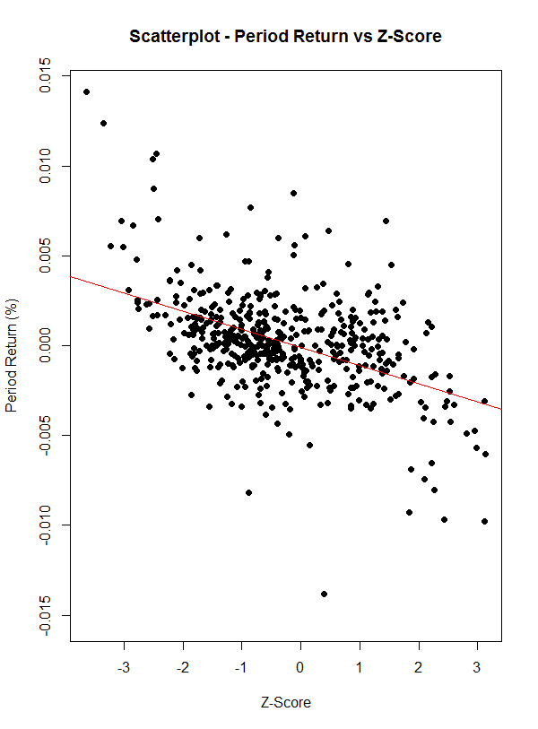
The stock price’s future period.return is the what we are after, and is therefore defined as the dependent variable. The explanatory variable(s) are the look-back columns and the z.score. You can plot a simple, one variable scatterplot to estimate the correlation between the z.score and the period.return.
# - graphing the correlations on the in-sample data
# - simple - period.return vs z-score
plot(in.samp[[1]]$z.score, in.samp[[1]]$period.return, main="Scatterplot - Period Return vs Z-Score", xlab = "Z-Score", ylab = "Period Return (%)",pch=19)
# Add fit lines
abline(lm(in.samp[[1]]$period.return~in.samp[[1]]$z.score), col="red") # regression line (y~x)
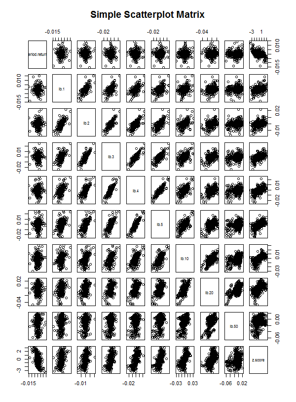
You can also view a correlation matrix to see all of the explanatory variable’s relationship (ie, each look-back column and the z.score) to see all of the correlations.
# - graph all correlations
pairs(~period.return+lb.1+lb.2+lb.3+lb.4+lb.5+lb.10+lb.20+lb.50+z.score,data=in.samp[[1]],
   main="Simple Scatterplot Matrix")
Then you can run the model on the in-sample or test data, and apply it to the out-of-sample data using the predict() function. You can measure the accuracy of the predicted values to the actual values of the out-of-sample data by using the accuracy() function.
# - applying multiple linear regression to the in-sample data, use the returns over the past 10, 20 and 50 periods and the z.score to model the look-forward return over the future 20 periods)
mod.1 = lapply(in.samp,
          function(x)(
            lm(period.return~lb.1+lb.2+lb.3+lb.4+lb.5+lb.10+lb.20+lb.50+z.score, x) #
          )
        )
# - apply the model to the out-of sample data and return the fit and upper and lower prediction intervals (NOT confidence intervals)
pred.1 = lapply(seq_along(mod.1),
          function(x)(
            predict(mod.1[[x]], newdata = out.samp[[x]], interval = "prediction")
          )
        )
# - evaluate the accuracy of the model (the lower the mae, rmse, the better)
myaccuracy.1 = lapply(seq_along(pred.1),
                  function(x)(
                    accuracy(pred.1[[x]][,1],out.samp[[x]]$period.return)
                  )
                )
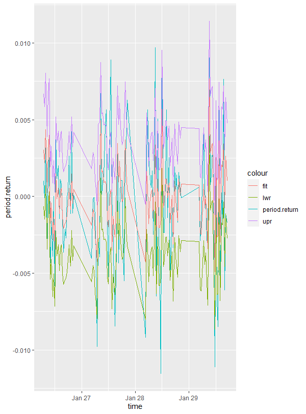
You can then graph the predicted values of the out-of-sample data versus the actual values of the out-of-sample data. The code below also adds upper and lower confidence limits for the predicted values.
# - graph the predicted return, actual return and upper and lower limits for
mydata = cbind(out.samp[[1]][1:120,],pred.1[[1]][1:120,])
ggplot(mydata, aes(x = time)) +
    geom_line(aes(y = period.return, colour = "period.return")) +
    geom_line(aes(y = fit, colour = "fit")) +
    geom_line(aes(y = upr, colour = "upr")) +
    geom_line(aes(y = lwr, colour = "lwr"))
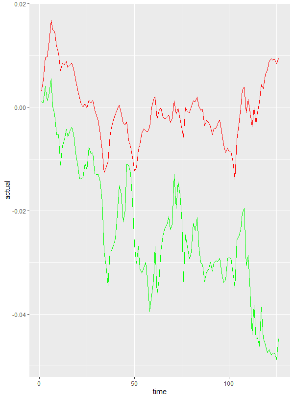
The above code in this section doesn’t attempt to create a trading system from the linear regression model. That is for another post sometime, and more work is definitely required. You can see that, even with the accuracy of the model, plotting the cumulative sum of the actual returns for the model (below in green) vs the cumulative sum of the predicted returns (below in red) reveals fairly large gaps. One solution is to use lm() to predict the look-forward columns. Again, for a future post!
Thank you for reading, and happy R-ing!
Notes and Research
-
[21 Iteration R for Data Science](https://r4ds.had.co.nz/iteration.html) -
[Use Z-Scores To Maximize Your Portfolio’s Potential Seeking Alpha](https://seekingalpha.com/article/3224666-use-z-scores-to-maximize-your-portfolios-potential) - PerformanceAnalytics.pdf
- Performance Analysis with tidyquant • tidyquant
- Z-Score: Definition, Formula and Calculation - Statistics How To
- Using BatchGetSymbols to download financial data for several tickers
-
[Download historical data in Yahoo Finance Yahoo Help - SLN2311](https://help.yahoo.com/kb/download-historical-data-yahoo-finance-sln2311.html) -
[Quartiles, Deciles, and Percentiles R-bloggers](https://www.r-bloggers.com/2013/06/quartiles-deciles-and-percentiles/) - Linear Regression Example in R using lm() Function – Learn by Marketing
- Predict in R: Model Predictions and Confidence Intervals - Articles - STHDA
-
[rollapply function R Documentation](https://www.rdocumentation.org/packages/zoo/versions/1.8-8/topics/rollapply) - Tests of Statistical Significance
-
[Validation Methods For Trading Strategy Development by Michael Harris Towards Data Science](https://towardsdatascience.com/validation-methods-for-trading-strategy-development-1efea8284b02) -
[Demystifying Statistical Analysis 2: The Independent t-Test Expressed in Linear Regression by The Curious Learner Medium](https://medium.com/@wyess/demystifying-statistical-analysis-2-the-independent-t-test-expressed-in-linear-regression-434a3b302289) - Predict in R: Model Predictions and Confidence Intervals - Articles - STHDA
- Predicting Stock Market Returns
- Other Information
- DMwR In Class - Predicting Stock Market Returns
- Stock Market Prediction with R - Stock Price Prediction Project
- r - Plotting two variables as lines using ggplot2 on the same graph - Stack Overflow
-
[Mean Reversion: Simple Trading Strategies Part 1 by Auquan auquan Medium](https://medium.com/auquan/mean-reversion-simple-trading-strategies-part-1-a18a87c1196a) - Plot graphs in R by loop and save it like jpeg - Stack Overflow
- Multivariate Linear Regression
-
[What does RMSE really mean?. Root Mean Square Error (RMSE) is a… by James Moody Towards Data Science](https://towardsdatascience.com/what-does-rmse-really-mean-806b65f2e48e) -
[Measuring forecast model accuracy to optimize your business objectives with Amazon Forecast AWS Machine Learning Blog](https://aws.amazon.com/blogs/machine-learning/measuring-forecast-model-accuracy-to-optimize-your-business-objectives-with-amazon-forecast/) -
[3.4 Evaluating forecast accuracy Forecasting: Principles and Practice (2nd ed)](https://otexts.com/fpp2/accuracy.html) - accuracy function - RDocumentation
- Time Series Forecasting Performance Measures With Python
- R: How to create, delete, move, and more with files - Open Source Automation
- Python File Write