Creating a Martingale Trading System
Introduction
This blog post will attempt to create a Martingale-type trading system.
Martingale systems are famous (or infamous) styles of betting that instructs a bettor to increase bets after each individual loss in hopes that an eventual “big” win will recover all previous losses. The classic example is a fair coin-flip where a heads or tails offers a 50% probability of success. The gambler doubles his bet after each loss and bets the same amount (typically 1-unit) after each win.
The Anti-Martingale System is the opposite. In the fair coin flip example, the bettor doubles the bet after each win and decreases (usually by half) the bet size after a loss.
Criticism of both systems fall squarely on the gambler’s fallacy or “the incorrect belief that, if a particular event occurs more frequently than normal during the past, it is less likely to happen in the future (or vice versa), when it has otherwise been established that the probability of such events does not depend on what has happened in the past.” In statistical terms, each coin flip is statistically independent of the last; in a fair coin flip, whether a heads or tails comes up next is not dependent on the outcome of the previous coin flip.
The question this blog post attempts to answer is whether consecutive up-days or down-days make it more or less likely for the stock to have an opposite move the following day. And if it is more likely for a stock to change direction, whether a profitable system can be created from that knowledge.
Account Size and Roulette
Practical matters are also at play with Martingale. An adequate account is required, and has an effect on Martingale systems’ performance when betting or trading. Doubling a bet at a roulette table in a casino can cause a player to either come up against table limits or simply run out of money to bet when there is an occurrence of consecutive losses. For example, “[t]o have an under 10% chance of failing to survive a long loss streak during 5,000 plays, the bettor must have enough to double their bets for 15 losses. This means the bettor must have over 65,500 (2^15-1 for their 15 losses and 2^15 for their 16th streak-ending winning bet) times their original bet size. Thus, a player making 10 bets would want to have over 655,000 in their bankroll (and still have a ~5.5% chance of losing it all during 5,000 plays).”
You can prove this last statement with a couple of lines of R code. Note that this article uses “streaks” and “runs” interchangeably to refer to a consecutive occurrence of wins and/or losses.
set.seed(8675)

# - 100k spins where 0 = win for player and 1 = win for house
# - player wins 45% of the time and house wins 55% of the time
roulette_spins <- sample(c(0,1),100000,replace = T, prob = c(.45,.55))

# - calculate player and house wins and house winning percentage
player_wins <- length(roulette_spins[roulette_spins == 0])
house_wins <- length(roulette_spins[roulette_spins == 1])
house_wp <- house_wins/(player_wins + house_wins)

# - find the consecutive runs
roulette_runs <- rle(roulette_spins)

# - data frame shoing the occurrences of consecutive runs and the pct of total each occurs for player and house
unique_runs_player <- as.data.frame(table(roulette_runs$lengths[roulette_runs$values == 0]))
  unique_runs_player <- unique_runs_player %>% mutate(pct = round(Freq/(sum(unique_runs_player$Freq)),4))
unique_runs_house <- as.data.frame(table(roulette_runs$lengths[roulette_runs$values == 1]))
  unique_runs_house <- unique_runs_house %>% mutate(pct = round(Freq/(sum(unique_runs_house$Freq)),4))
print(house_wp)
## [1] 0.55094
The house winning percentage is around 55% based on 100,000 spins of the
wheel. This is the “house advantage” I programmed in for the prob
variable using the sample() function.
print(unique_runs_player)
##    Var1  Freq    pct
## 1     1 13615 0.5513
## 2     2  6122 0.2479
## 3     3  2643 0.1070
## 4     4  1283 0.0520
## 5     5   581 0.0235
## 6     6   260 0.0105
## 7     7    93 0.0038
## 8     8    56 0.0023
## 9     9    21 0.0009
## 10   10    13 0.0005
## 11   11     7 0.0003
## 12   13     2 0.0001
For the player, there were only 2 occasions out of 100,000 where 13 wins in a row occurred.
print(unique_runs_house)
##    Var1  Freq    pct
## 1     1 10970 0.4442
## 2     2  6194 0.2508
## 3     3  3393 0.1374
## 4     4  1886 0.0764
## 5     5  1009 0.0409
## 6     6   573 0.0232
## 7     7   314 0.0127
## 8     8   157 0.0064
## 9     9    86 0.0035
## 10   10    48 0.0019
## 11   11    26 0.0011
## 12   12    17 0.0007
## 13   13    11 0.0004
## 14   14     5 0.0002
## 15   15     3 0.0001
## 16   17     2 0.0001
## 17   19     1 0.0000
## 18   21     1 0.0000
But the house advantage starts to shine through. In our scenario, the house had 15 consecutive wins on 3 occurrences and 19 & 21 consecutive wins on 1 occurrence during the 100,000 spins. As referenced above, a 10-dollar bettor who is unlucky enough to have 19 losses in a row would lose 2^21-1 * $10 or $2,097,142 during this brutal stretch. Ouch!
Load Libraries & Get Data
First, download the stock data. I used the tidyquant package to download multiple symbols.
# - list of symbols to analyze
p.symbol <- c("AAPL", "SPY", "QQQ", "CSCO", "F", "AMZN", "AMD", "BAC", "T", "MU")

# - starting date for data
p.start <- "2015-01-01"

# - ending date for data
p.end <- "2022-06-01"

# - Get stock prices for multiple stocks
mult_stocks <- tq_get(p.symbol,
  get  = "stock.prices",
  from = p.start,
  to   = p.end
)

# - create a list of all stocks by symbol
df.data <- lapply(p.symbol, function(x) (mult_stocks %>% filter(symbol == x)))
Calculate Returns and Consecutive Up- and Down-Days
Next, we want to calculate the returns for each stock from
close-to-close and determine if each day was an “up-day” (returns are
greater than zero) or a “down-day” (returns are less than zero). This is
shown in the my.dir column below where a 1 is an up-day and a 0 is
a down-day.
# - add returns and up/down column
df.data.2 <-
  lapply(df.data, function(x) {
    (
      x %>% mutate(
        my.ret = adjusted / lag(adjusted, n = 1) - 1,
        my.dir = ifelse(my.ret > 0, 1, 0)
      )
    )
  })

# - remove any columns with NA returns
df.data.3 <- lapply(df.data.2, function(x) (x[!is.na(x$my.ret), ]))
What is central to Martingale and Anti-Martingale systems is the number
of consecutive up and down periods (in this case days) of a given stock.
This can be found using the rle() function in base R. Using the
my.dir column above, we can calculate the number of times the stock
had a consecutive up-day or down-day. In rle() nomenclature, a
length is the number of consecutive equal values in a
vector.
A vector c(1,1,1,1,1,1) would have a run with a value of 1 and
length equal to 6. You can think of the length as a streak of up or
down-days.
# - custom function to return a list of data.frames for each value
fn.show.run.data <- function(df) {
  # - solve for the number of runs for each stock
  df <- rle(df$my.dir)

  # - solve for min and max lengths of runs and unique values and lengths
  my.min <- max(min(df$lengths), 1)
  my.max <- max(df$lengths)
  my.vals <- unique(df$values)
  my.lens <- sort(unique(df$lengths))

  # - returns a list for all valuse for each individual length of occurrent of a given run
  all.vals <- lapply(my.min:my.max, function(x) (length(which(df$lengths == x))))

  # - convert list to data.frame
  df.all.vals <- list(data.frame(
    my.vals = NA,
    my.lens = my.min:my.max,
    my.runs = unlist(all.vals),
    cum.runs = cumsum(unlist(all.vals)),
    cum.runs.pct = round(cumsum(unlist(all.vals)) / sum(unlist(all.vals)), 2)
  ))

  # - returns a list by each value (ie, 0,1) for each individual length or occurrences of a given run (ie, 1:12)
  count.vals <- lapply(my.vals, function(x) {
    (
      lapply(my.min:my.max, function(y) {
        (
          length(which(df$lengths == y & df$values == x))
        )
      })
    )
  })

  # - convert list to data.frame by my.vals
  df.count.vals <- lapply(seq_along(my.vals), function(x) {
    (
      data.frame(
        my.vals = my.vals[[x]],
        my.lens = my.min:my.max,
        my.runs = unlist(count.vals[[x]]),
        cum.runs = cumsum(unlist(count.vals[[x]])),
        cum.runs.pct = round(cumsum(unlist(count.vals[[x]])) / sum(unlist(count.vals[[x]])), 2)
      )
    )
  })

  len <- length(my.vals) + 1
  my.return.list <- vector(mode = "list", length = len)

  for (i in 1:len) {
    if (i == 1) {
      my.return.list[i] <- df.all.vals[i]
    } else {
      my.return.list[i] <- df.count.vals[i - 1]
    }
  }

  # names(my.return.list) <- c("all_values",paste0("value_",my.vals))

  return(my.return.list)
}
To help understand runs a little better in relationship to consecutive
up and down days, let’s take a look at SPY data and apply the custom
function from above. The function returns a list of data.frames for
the second stock on our list which is SPY.
example.runs <- fn.show.run.data(df.data.3[[2]])
The first element on the list shows the statistics for all up- and down-days.
# - returns a data.frame with statistics for BOTH up and down days
example.runs[[1]]
##    my.vals my.lens my.runs cum.runs cum.runs.pct
## 1       NA       1     503      503         0.52
## 2       NA       2     234      737         0.76
## 3       NA       3     125      862         0.89
## 4       NA       4      58      920         0.95
## 5       NA       5      26      946         0.98
## 6       NA       6      12      958         0.99
## 7       NA       7       6      964         0.99
## 8       NA       8       4      968         1.00
## 9       NA       9       0      968         1.00
## 10      NA      10       0      968         1.00
## 11      NA      11       1      969         1.00
The second entry on the list shows the stats on down-days. You can
tell it is a down day since all entries in the my.vals column are
zeroes. For this example, there were 10 times when SPY had 5 consecutive
down-days. However, 97% of the consecutive down-days were 4 or less.
example.runs[[2]]
##    my.vals my.lens my.runs cum.runs cum.runs.pct
## 1        0       1     275      275         0.57
## 2        0       2     124      399         0.82
## 3        0       3      48      447         0.92
## 4        0       4      23      470         0.97
## 5        0       5      10      480         0.99
## 6        0       6       3      483         1.00
## 7        0       7       1      484         1.00
## 8        0       8       1      485         1.00
## 9        0       9       0      485         1.00
## 10       0      10       0      485         1.00
## 11       0      11       0      485         1.00
The third entry on the list shows the stats on up-days. Again, the
my.val column is all “1’s” indicating an up-day. SPY had 9 occurrences
of 6 consecutive up-days. However, 93% of the consecutive up days were 4
or less.
example.runs[[3]]
##    my.vals my.lens my.runs cum.runs cum.runs.pct
## 1        1       1     228      228         0.47
## 2        1       2     110      338         0.70
## 3        1       3      77      415         0.86
## 4        1       4      35      450         0.93
## 5        1       5      16      466         0.96
## 6        1       6       9      475         0.98
## 7        1       7       5      480         0.99
## 8        1       8       3      483         1.00
## 9        1       9       0      483         1.00
## 10       1      10       0      483         1.00
## 11       1      11       1      484         1.00
Let’s look at all of stocks and see what the runs look like.
# - apply custom function to all data
df.all.run.data <- lapply(df.data.3, fn.show.run.data) %>% bind_rows()

# - all days (where my.vals = 0 or 1)
df.all.run.data.all <-
  df.all.run.data %>%
  filter(my.vals != 0 | my.vals != 1) %>%
  group_by(my.lens) %>%
  summarize(
    sum = sum(my.runs)
  ) %>%
  mutate(
    cum.runs = cumsum(sum),
    cum.runs.pct = round(cum.runs / sum(sum) * 100, 2)
  )

colnames(df.all.run.data.all) <- c("my.lens", "my.runs", "cum.runs", "cum.runs.pct")

# - down days (where my.vals = 0)
df.all.run.data.down <-
  df.all.run.data %>%
  filter(my.vals == 0) %>%
  group_by(my.lens) %>%
  summarize(
    sum = sum(my.runs)
  ) %>%
  mutate(
    cum.runs = cumsum(sum),
    cum.runs.pct = round(cum.runs / sum(sum) * 100, 2)
  )

colnames(df.all.run.data.down) <- c("my.lens", "my.runs", "cum.runs", "cum.runs.pct")

# - up days (where my.vals = 1)
df.all.run.data.up <-
  df.all.run.data %>%
  filter(my.vals == 1) %>%
  group_by(my.lens) %>%
  summarize(
    sum = sum(my.runs)
  ) %>%
  mutate(
    cum.runs = cumsum(sum),
    cum.runs.pct = round(cum.runs / sum(sum) * 100, 2)
  )

colnames(df.all.run.data.up) <- c("my.lens", "my.runs", "cum.runs", "cum.runs.pct")
# - summary of all days
df.all.run.data.all
## # A tibble: 11 × 4
##    my.lens my.runs cum.runs cum.runs.pct
##      <int>   <int>    <int>        <dbl>
##  1       1    4838     4838         50.9
##  2       2    2359     7197         75.7
##  3       3    1202     8399         88.3
##  4       4     565     8964         94.3
##  5       5     290     9254         97.3
##  6       6     135     9389         98.7
##  7       7      57     9446         99.3
##  8       8      29     9475         99.6
##  9       9      21     9496         99.8
## 10      10       6     9502         99.9
## 11      11       8     9510        100
To summarize the 10 stocks we looked at going back to 2015:
- All Days (both Up-Days and Down-Days) 94% of all days consist of 4 or fewer consecutive up or down days.
- Down-Days 95% of all down-days were 4 or less consecutively.
- Up-Days 93% of all up-days were 4 or less consecutively.
Martingale systems are dependent on being successful at some point in the future. You “double” the bet after a loss. Therefore, it is important to have an idea regarding how many losses there might be in a row. This affects your “wager”.
A Simple Martingale System
To keep it simple, assume that you buy a stock at the close of each day and sell the stock at the close the following day, with the view that the price will be higher.
One simple way to test this type of Martingale system is to write a long-only function with the following rules:
- Wins Close existing position(s). Long 1-unit if period before was an up-day,
- Losses Close existing position(s). Long 2^Nth units if N-periods before was a down-day.
“N” in the expression above is the number of consecutive down-days. So if yesterday was the 3rd down-day in a row, you would be long 2^3 units for today.
A few notes about the assumptions of the Simple Martingale system:
- You can buy and sell exactly at the close. You can draw your own conclusions to the reality of this, but for the purposes of this post, that is my assumption. There is also no slippage or commission costs included. You can add those, should you so choose.
- It is assumed a new position is exited and entered at each close. Long and it is an up-day? Sell-to-close the current 1-unit position and buy-to-open another 1-unit position at the close. If you are long and it is the 3rd consecutive down-day? Sell-to-close your current position (which is 4-units) and buy-to-open a new 8-unit position. Again, both are entered at the closing price.
- For ease of reference, 1-unit is equal to 1-share of the stock.
# - add column showing cumulative up/down days
df.data.4 <- lapply(df.data.3, function(x) {
  (
    x %>% mutate(
      # - add column showing cumulative up/down days
      cum.my.dir = with(rle(my.dir), sequence(lengths)),
      # - add column showing number of units based on consecutive runs
      my.units = ifelse(lag(my.dir, 1) == 1, 1, 2^lag(cum.my.dir, 1)),
      # - add column - share $ price made/lost on trade
      my.shares = (adjusted - lag(adjusted, 1)) * my.units,
      tot_ret = (adjusted - lag(adjusted, 1)) / adjusted * my.units,
      cum_ret = cumprod(ifelse(1:n() == 1, 1, tot_ret + 1)) - 1
      )
  )
})

df.data.4 <- lapply(df.data.4, function(x) (x[!is.na(x$my.units), ]))

# - add column showing cumulative position
df.data.5 <- lapply(df.data.4, function(x) (x %>% mutate(cum.my.shares = cumsum(my.shares))))
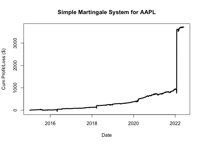
Let’s take a look at the first two stocks and how they performed.
# - plot the first symbol
plot(df.data.5[[1]]$date, df.data.5[[1]]$cum.my.shares, type = "l", lwd = 3, main = paste("Simple Martingale System for", p.symbol[[1]]), xlab = "Date", ylab = "Cum Profit/Loss ($)")
# - plot the second symbol
plot(df.data.5[[2]]$date, df.data.5[[2]]$cum.my.shares, type = "l", lwd = 3, main = paste("Simple Martingale System for", p.symbol[[2]]), xlab = "Date", ylab = "Cum Profit/Loss ($)")
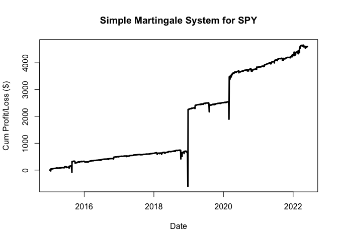
The graphs are encouraging but there are a couple of big jumps AND big drawdowns. Let’s look a little deeper with some common trading system analytics.
# - function to calculate the total $ value drawdown (peak to trough)
# - adapted from https://stackoverflow.com/questions/13733166/maxdrawdown-function
fn.drawdown <- function(pnl) {
  cum.pnl <- c(0, cumsum(pnl))
  drawdown <- cum.pnl - cummax(cum.pnl)
  return(tail(drawdown, -1))
}

# - function to find the MAX drawdown
fn.max.drawdown <- function(pnl) {
  cum.pnl <- c(0, cumsum(pnl))
  drawdown <- cum.pnl - cummax(cum.pnl)
  maxdraw <- min(tail(drawdown, -1))
  return(maxdraw)
}

# - calculate trade stats for each stock
df.trade.stats <-
  lapply(seq_along(df.data.5), function(x) {
    (
      data.frame(
        net_profit = sum(df.data.5[[x]]$my.shares, na.rm = T),
        wins = length(which(df.data.5[[x]]$my.shares > 0)),
        loss = length(which(df.data.5[[x]]$my.shares < 0)),
        win_percent = round(length(which(df.data.5[[x]]$my.shares > 0)) / (length(which(df.data.5[[x]]$my.shares > 0)) + length(which(df.data.5[[x]]$my.shares < 0))), 4) * 100,
        max_val = max(df.data.5[[x]]$cum.my.shares),
        min_val = min(df.data.5[[x]]$cum.my.shares),
        max_draw = fn.max.drawdown(df.data.5[[x]]$my.shares),
        max_shares = max(df.data.5[[x]]$my.units)
      )
    )
  })

# - combine list to data.frame and add symbols
df.trade.stats.2 <- rbindlist(df.trade.stats) %>%
  round(., 2) %>%
  add_column(p.symbol)

# - view all trade stats for each symbol
df.trade.stats.2
##     net_profit wins loss win_percent max_val min_val max_draw max_shares
##  1:    3716.77  987  874       53.04 3719.75  -48.08  -191.15        256
##  2:    4606.61 1023  837       55.00 4658.26 -600.72 -1345.33        256
##  3:    2827.99 1053  807       56.61 2828.80  -68.16  -405.65        512
##  4:     325.25  976  867       52.96  450.66  -76.24  -236.06        512
##  5:     213.16  900  921       49.42  219.13  -19.88   -81.91        256
##  6:    1413.62 1008  855       54.11 1445.24  -24.79  -591.87        256
##  7:     426.18  950  873       52.11  951.89 -386.10 -1337.99        256
##  8:     273.97  949  887       51.69  327.19  -21.23  -202.60        512
##  9:     741.81  973  869       52.82  741.84  -10.70   -45.00        512
## 10:     651.31  958  892       51.78  651.31 -117.70  -269.47        512
##     p.symbol
##  1:     AAPL
##  2:      SPY
##  3:      QQQ
##  4:     CSCO
##  5:        F
##  6:     AMZN
##  7:      AMD
##  8:      BAC
##  9:        T
## 10:       MU
# - summary (mean) of all trade stats columns
df.trade.stats.2.summ <- apply(rbindlist(df.trade.stats), 2, function(x) (mean(x, na.rm = T))) %>% round(., 2)

# - view summary for all symbols
df.trade.stats.2.summ
##  net_profit        wins        loss win_percent     max_val     min_val
##     1519.67      977.70      868.20       52.95     1599.41     -137.36
##    max_draw  max_shares
##     -470.70      384.00
Notes on the Simple Martingale System
Although the system looks fairly profitable, it has its limitations. The main issue that systems like these run into is that up-days and down-days are not symmetrical. The coin-flip assumptions always return 1:1; a 1-dollar bet results in either a 1-dollar win or loss. In stocks, an up-day might be a 2% increase in the stock price, while a down-day is a 4% decrease. This asymmetry of returns causes the basic assumption of the system (ie, bet double after a loss) to fail.
One “fix” would be to compartmentalize the returns into buckets such that instead of taking profits at a given time you take profits or double-down at a given return. For example, take profits and put on a new position at a +1% return. If price decreases to -1%, sell to close and buy 2-units with a new +1% profit target.
Reverse Martingale
Anti- or Reverse Martingale is, well, the opposite of a Martingale system. Instead of betting one-unit after a win and doubling your bet after each loss, you double your bet after each win and reduce your bet size after a loss.
A long-only Reverse Martingale function could be stated as follows:
- Losses: Close existing position(s). Long 1-unit if period before was a down-day.
- Wins: Close existing position(s). Long 2^Nth units if N-periods before was an up-day.
The same assumptions for the Simple Martingale regarding trade entry and exit are used.
# - add column showing cumulative up/down days
df.data.6 <- lapply(df.data.3, function(x) {
  (
    x %>% mutate(
      # - add column showing cumulative up/down days
      cum.my.dir = with(rle(my.dir), sequence(lengths)),
      # - add column showing number of units based on consecutive runs
      my.units = ifelse(lag(my.dir, 1) == 1, 2^lag(cum.my.dir, 1), 1),
      # - add column - share $ price made/lost on trade
      my.shares = (adjusted - lag(adjusted, 1)) * my.units,
      tot_ret = my.units * my.ret,
      cum_ret = cumprod(ifelse(1:n() == 1, 1, tot_ret + 1)) - 1
    )
  )
})

df.data.7 <- lapply(df.data.6, function(x) (x[!is.na(x$my.units), ]))

# - add column showing cumulative position
df.data.8 <- lapply(df.data.7, function(x) (x %>% mutate(cum.my.shares = cumsum(my.shares))))
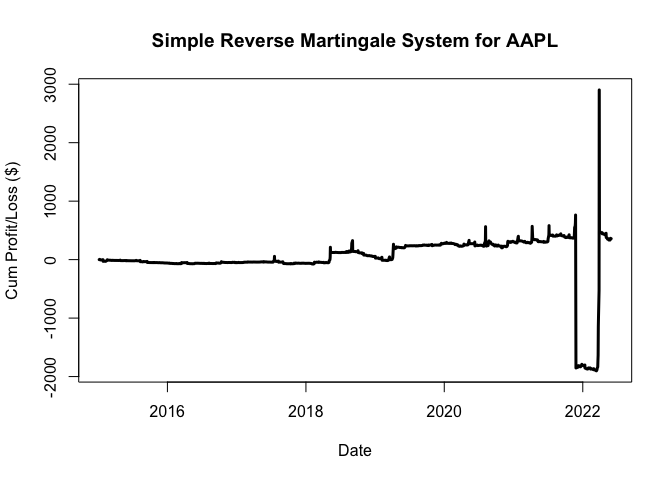
Once again, plot the first two stocks and how they performed.
# - plot the first symbol
plot(df.data.8[[1]]$date, df.data.8[[1]]$cum.my.shares, type = "l", lwd = 3, main = paste("Simple Reverse Martingale System for", p.symbol[[1]]), xlab = "Date", ylab = "Cum Profit/Loss ($)")
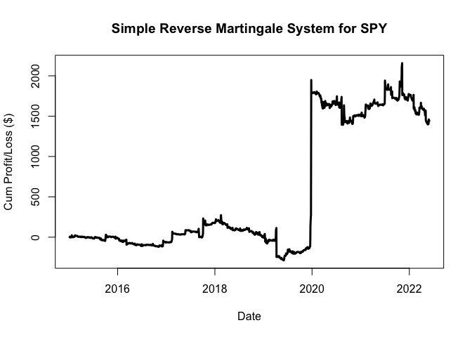
# - plot the second symbol
plot(df.data.8[[3]]$date, df.data.8[[2]]$cum.my.shares, type = "l", lwd = 3, main = paste("Simple Reverse Martingale System for", p.symbol[[2]]), xlab = "Date", ylab = "Cum Profit/Loss ($)")
Trade stats for the Simple Reverse Martingale system:
df.trade.stats.3 <-
  lapply(seq_along(df.data.8), function(x) {
    (
      data.frame(
        net_profit = sum(df.data.8[[x]]$my.shares, na.rm = T),
        wins = length(which(df.data.8[[x]]$my.shares > 0)),
        loss = length(which(df.data.8[[x]]$my.shares < 0)),
        win_percent = round(length(which(df.data.8[[x]]$my.shares > 0)) / (length(which(df.data.8[[x]]$my.shares > 0)) + length(which(df.data.8[[x]]$my.shares < 0))), 4) * 100,
        max_val = max(df.data.8[[x]]$cum.my.shares),
        min_val = min(df.data.8[[x]]$cum.my.shares),
        max_draw = fn.max.drawdown(df.data.8[[x]]$my.shares),
        max_shares = max(df.data.8[[x]]$my.units)
      )
    )
  })

df.trade.stats.4 <- rbindlist(df.trade.stats.3) %>%
  round(., 2) %>%
  add_column(p.symbol)

df.trade.stats.4
##     net_profit wins loss win_percent max_val   min_val  max_draw max_shares
##  1:     358.58  987  874       53.04 2901.72  -1902.13  -2664.74       2048
##  2:    1440.91 1023  837       55.00 2156.84   -287.26   -758.90       2048
##  3:   -9018.09 1053  807       56.61 4360.51 -10212.66 -14573.17       2048
##  4:     414.07  976  867       52.96  718.51    -15.77   -309.47       2048
##  5:    -471.89  900  921       49.42   66.14   -504.07   -570.21       1024
##  6:     833.73 1008  855       54.11 1709.96    -24.42   -944.29        512
##  7:    -268.82  950  873       52.11  777.67   -293.35  -1071.02        512
##  8:     321.51  949  887       51.69  448.67    -70.78   -178.59       2048
##  9:     171.56  973  869       52.82  463.96    -72.57   -296.78       1024
## 10:    -710.46  958  892       51.78  547.31   -732.17  -1279.48       2048
##     p.symbol
##  1:     AAPL
##  2:      SPY
##  3:      QQQ
##  4:     CSCO
##  5:        F
##  6:     AMZN
##  7:      AMD
##  8:      BAC
##  9:        T
## 10:       MU
df.trade.stats.4.summ <- apply(rbindlist(df.trade.stats.3), 2, function(x) (mean(x, na.rm = T))) %>% round(., 2)

df.trade.stats.4.summ
##  net_profit        wins        loss win_percent     max_val     min_val
##     -692.89      977.70      868.20       52.95     1415.13    -1411.52
##    max_draw  max_shares
##    -2264.67     1536.00
Interestingly, win percentage for the Martingale and Anti-Martingale are the same. But this was to be expected. Recall that both systems are long only. The only thing we are changing is the profit target albeit in an indirect manner through the amount of exposure we have to each stock. The stock goes up or down the same amount from close to close, and since you are long for both strategies, a win (whether the stock was higher after 1-day) is the same. The only difference his how many shares of stock or units you are long. This is where the profits and loss accrue. In that way, Martingale and Anti Martingale are really position sizing systems rather than a true trading system based on probability or statistics.
Anti-Martingale systems look so much worse because of an inherent tendency to bet biggest long when it is least likely another up-day will occur.
To simplify this point, look back at the table above showing all up-days for all 10 of our stocks. If you are on the 5th straight up-day in an Anti-Martingale system, the system says to bet 2^5 or 32 units. Out of 4752 up-days across all stocks I measured, a 6th consecutive up-day only occurred 71 times or about 1.5%. Anti-Martingale says bet 32x normal when there is historically only a 1.5% chance of a win; at some point, the odds catch up with you.
The flip side is also true. Martingale says bet biggest when the odds of a reversal are (historically) on your side. In our example scenario, if you are on the 5th straight down-day, Martingale says to get long the same 32 units. But the odds of a 6th straight down day is 55/4729 or 1.2% meaning that there is an almost 98.8% chance of an up day. Martingale gets a bad name for doubling down when you are down and not letting profits run, but the historical odds are actually on Martingale’s side. The further a streak goes, the less likely it is to continue allowing the trader to claw out of the hole they are in and ride the next winning streak.
Hybrid Martingale System
What if you could take the best parts of the Martingale and Anti-Martingale Systems and combine them? Based on our 1-share position-size system, Martingale trade systems advantage over Reverse Martingale trade systems can be summarized as follows:
- Low Drawdowns. The mean drawdown for all ten stocks was $476 for the Martingale versus $3366 for the Anti-Martingale. That is a 1 to 7 ratio; for every dollar Martingale lost, Anti-Martingale lost 7 dollars.
- Fewer Shares. Martingale maxed out at 512 shares with an average of 345 shares held. Reverse Martingale had several stocks that traded 2048 shares with an average of 1536 shares held. This is likely due to the number of consecutive down days that each stock experienced in comparison to consecutive up days.
- Smaller Account Size. This is a corollary of lower drawdowns and fewer shares traded. Martingale would require a much smaller account size than Anti-Martingale.
An Alternate Take: Replicating An Article’s Martingale Strategy
An article on Martingale and Reverse Martingale strategies proposed a similar simple framework for evaluating both types of systems on 6-months of AAPL stock. The main difference between what I proposed so far, versus the article’s strategy was how the author accounted for an up-day and a down-day for the daily price data.
- An up-day was defined as when the close of the day was 2% greater than the prior day
- A down-day was when the close was 2% less than the prior day.
In other words, the long position was never closed and profits were never realized day-to-day.
Instead, double the number of shares are purchased and added to the account following a down-day, and no additional shares are added following an up-day. This results in larger position sizes compared with my original Martingale strategy since:
- you don’t exit the position and re-enter single unit on up-days, and
- you don’t exit open positions and re-enter 2^N units following a consecutive down days.
Below is the article’s Martingale Strategy Python code recreated in R
using the first 125 days of AAPL stock.
# - get first 100 data points from first symbol
art.data <- df.data[[1]][1:125, ]

# - extract date and adjusted close price
# - add daily close to close percentage returns, long_signal (increase of 2% from prior day), short signal (decrease 2%), combined signal
df.article <- art.data[, c(2, 8)] %>%
  mutate(
    ret = adjusted / lag(adjusted, 1) - 1,
    long_signal = ifelse(adjusted > 1.02 * lag(adjusted, 1), 1, 0),
    short_signal = ifelse(adjusted < .98 * lag(adjusted, 1), -1, 0),
    signal = long_signal + short_signal
  )

# - loop to create vector "df.article.2" that adds 2 shares every time there is a loss of 2%

# - create an empty vector with length equal to number of rows of df.article
df.article.2 <- rep(NA, nrow(df.article))

# - for-loop to calculate the quantity of shares owned
# - note that the system starts with 1 share
for (i in 1:nrow(df.article)) {
  if (i == 1) {
    df.article.2[1] <- 1
  } else {
    if (df.article$signal[i] == 1) {
      df.article.2[i] <- df.article.2[i - 1]
    }
    if (df.article$signal[i] == -1) {
      df.article.2[i] <- df.article.2[i - 1] * 2
    }
    if (df.article$signal[i] == 0) {
      df.article.2[i] <- df.article.2[i - 1]
    }
  }
}

# - add the quantity column to the original data.frame
df.article.3 <- df.article %>% add_column(quantity = df.article.2)

# - add a tot_return column
# - tot_return calculated by taking the ret (daily return) times the quantity of shares purchased
df.article.4 <- df.article.3 %>% mutate(
  acct_val = adjusted * quantity,
  tot_ret = (adjusted - lag(adjusted, 1)) / adjusted * quantity,
  cum_ret = cumprod(ifelse(row_number(df.article.3$date) == 1, 1, tot_ret + 1)) - 1
)
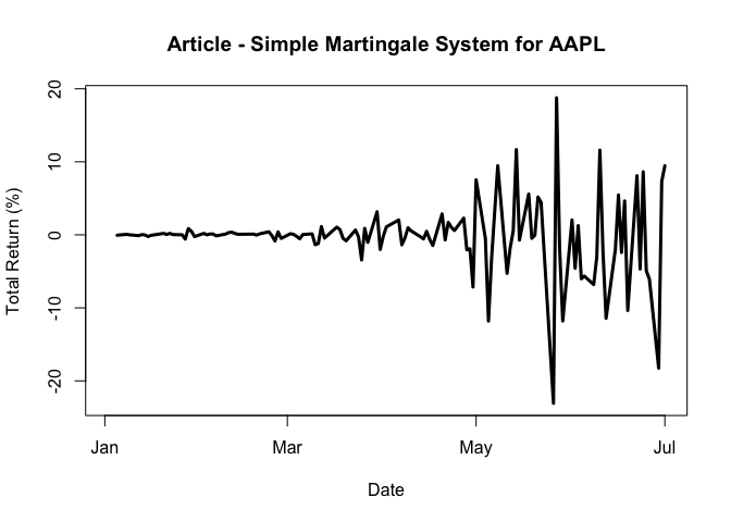
Plot the returns using the article’s Simple Martingale Strategy.
# - plot article returns - Martingale Strategy
plot(df.article.4$date, df.article.4$tot_ret, type = "l", lwd = 3, main = paste("Article - Simple Martingale System for", p.symbol[[1]]), xlab = "Date", ylab = "Total Return (%)")
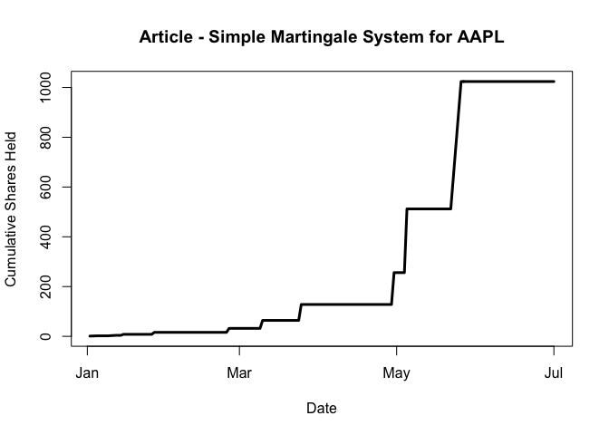
Plot the quantity held for the article’s Simple Martingale Strategy.
# - plot quantity - Martingale Strategy
plot(df.article.4$date, df.article.4$quantity, type = "l", lwd = 3, main = paste("Article - Simple Martingale System for", p.symbol[[1]]), xlab = "Date", ylab = "Cumulative Shares Held")
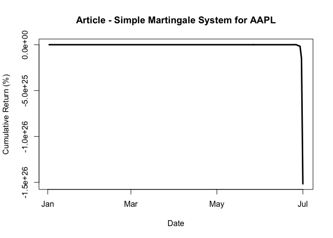
Plot the cumulative returns for the article’s Simple Martingale Strategy.
# - plot article cumulative returns
plot(df.article.4$date, df.article.4$cum_ret, type = "l", lwd = 3, main = paste("Article - Simple Martingale System for", p.symbol[[1]]), xlab = "Date", ylab = "Cumulative Return (%)")
Replicating An Article’s Reverse Martingale Strategy
I can also replicate the Reverse Martingale strategy from the
article. Note that we will use
the same data from the Martingale Strategy above. The signals
(represented in the data.frame df.article.2) will also stay the same.
For the Reverse Martingale strategy:
- a long signal is generated if the adjusted close changes by more than 2%, and
- a short signal is generated if the adjusted close decreases by 2% or more.
The only difference is that the system will double the trade size after a winning trade and halve the trade size after a losing trade.
# - loop to create vector "df.article.5" for Reverse Martingale strategy

# - create an empty vector with length equal to number of rows of df.article
df.article.5 <- rep(NA, nrow(df.article))

# - for-loop to calculate the quantity of shares owned
# - note that the system starts with 1 share
for (i in 1:nrow(df.article)) {
  if (i == 1) {
    df.article.5[1] <- 10
  } else {
    if (df.article$signal[i] == 1) {
      df.article.5[i] <- df.article.5[i - 1] * 2
    }
    if (df.article$signal[i] == -1) {
      df.article.5[i] <- df.article.5[i - 1] / 2
    }
    if (df.article$signal[i] == 0) {
      df.article.5[i] <- df.article.5[i - 1]
    }
  }
}

# - add the quantity column to the original data.frame
df.article.6 <- df.article %>% add_column(quantity = df.article.5)

# - add a tot_return column
# - tot_return calculated by taking the ret (daily return) times the quantity of shares purchased
df.article.7 <- df.article.6 %>% mutate(
  acct_val = adjusted * quantity,
  tot_ret = (adjusted - lag(adjusted, 1)) / adjusted * quantity,
  cum_ret = cumprod(ifelse(row_number(df.article.6$date) == 1, 1, tot_ret + 1)) - 1
)
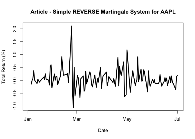
Plot the returns of the article’s Reverse Martingale Strategy.
# - plot article returns
plot(df.article.7$date, df.article.7$tot_ret, type = "l", lwd = 3, main = paste("Article - Simple REVERSE Martingale System for", p.symbol[[1]]), xlab = "Date", ylab = "Total Return (%)")
Plot the quantity held for the article’s Reverse Martingale strategy.
# - plot article quantity - Reverse Martingale strategy
plot(df.article.7$date, df.article.7$quantity, type = "l", lwd = 3, main = paste("Article - Simple REVERSE Martingale System for", p.symbol[[1]]), xlab = "Date", ylab = "Cumulative Shares Held")

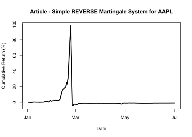
Plot the cumulative returns for the Reverse Martingale strategy.
# - plot article returns
plot(df.article.7$date, df.article.7$cum_ret, type = "l", lwd = 3, main = paste("Article - Simple REVERSE Martingale System for", p.symbol[[1]]), xlab = "Date", ylab = "Cumulative Return (%)")
Improvements on the Simple Martingale Strategy
The following improvements would likely improve the Martingale Strategy I created above.
Enter Only When Consecutive Days Equal 4 or More
One idea is to only enter a long position if there have been four or more consecutive down-days. Note that this approach assumes that:
- you continue to enter a NEW long position on the 5th, 6th, 7th etc. days assuming that days after the entry day are still down-days, and
- you purchase the appointed number of shares equal to 2^N-1.
For example, on the close of the 4th consecutive down-day, you purchase 8 units of stock. The next day, if the stock has its 5th consecutive down-day, you would both sell the 8 units and purchase 16 units at the close.
# - add a lead function (lookforward) showing the return 1-period (day) after the current period
# - filter for (1) consecutive days greater than 4 and (2) direction = down-day
df.data.9 <-
  lapply(df.data.5, function(x) {
    x %>% mutate(lf = lead(my.shares, n = 1)) %>% filter(cum.my.dir >= 4 & my.dir == 0)
  })

df.data.10 <- lapply(seq_along(df.data.9), function(x) {
  (
    data.frame(
      net_profit = sum(df.data.9[[x]]$lf, na.rm = T) * 100,
      wins = length(which(df.data.9[[x]]$lf > 0)),
      loss = length(which(df.data.9[[x]]$lf < 0)),
      win_percent = round(length(which(df.data.9[[x]]$lf > 0)) / (length(which(df.data.9[[x]]$lf > 0)) + length(which(df.data.9[[x]]$lf < 0))), 4) * 100,
      avg_win = sum(df.data.9[[x]]$lf[df.data.9[[x]]$lf > 0]) / length(df.data.9[[x]]$lf[df.data.9[[x]]$lf > 0]) * 100,
      avg_loss = sum(df.data.9[[x]]$lf[df.data.9[[x]]$lf < 0]) / length(df.data.9[[x]]$lf[df.data.9[[x]]$lf < 0]) * 100,
      avg_all = sum(df.data.9[[x]]$lf) / length(df.data.9[[x]]$lf) * 100
    )
  )
})

df.trade.stats.5 <- rbindlist(df.data.10) %>%
  round(., 2) %>%
  add_column(p.symbol)
df.trade.stats.5
##     net_profit wins loss win_percent  avg_win  avg_loss avg_all p.symbol
##  1:  329464.15   38   25       60.32  9789.69  -1701.76 5229.59     AAPL
##  2:  388905.16   38   23       62.30 18138.99 -13059.84 6375.49      SPY
##  3:  188502.99   33   27       55.00 10056.22  -5309.35 3141.72      QQQ
##  4:   15943.76   43   47       47.78  2685.74  -2117.94  175.21     CSCO
##  5:   21972.50   65   53       55.08   736.17   -488.27  183.10        F
##  6:  133968.87   48   28       63.16  5062.57  -3894.08 1762.75     AMZN
##  7:   -2336.01   57   32       64.04  2861.19  -5169.50  -25.39      AMD
##  8:   29415.69   57   46       55.34  1799.49  -1590.33  285.59      BAC
##  9:   74295.22   56   43       56.57  1682.55   -463.43  750.46        T
## 10:   46870.06   45   40       52.94  2502.63  -1643.70  545.00       MU
Focusing solely on win percentage, entering long after 4 or more consecutive down-days increased winning percentage average by 5% to 57.253 compared to 52.954 winning percentage for all down-days.
Other possible alternatives for improving the the strategies noted above include:
- For Reverse Martingale systems, set a maximum number of shares long to limit large positions.
- For both systems, exiting the long position and/or entering short after N number of consecutive up-days.
- Varying the units to reflect more granular buckets of gain and loss. Here, an up-day or a down-day was only evaluated at the close of the day. More frequent data would allow for a more exact measurement of up-periods and down-periods.
- Relate the up and down measurements to the actual stock returns rather than time. For example, first set a hypothetical “return bucket” (ie, the percentage the stock changed in a given time period) to .10% based on 1-minute data. Then you could measure the runs based off of the return bucket, rather than on time. This is similar to using range bars.
- Relate runs to returns and implement some type of position management system. If I told you there was a 24.2% chance of a stock having a down-day the next day, how much would you bet that this would come true? It’s hard to answer that question because you don’t know what you would get in return. You obviously would not take an even bet; this would have a negative expectation. In reality, you would want to get more than 3.1-to-1 on your money to make it worth your while. Consecutive run percentages are no different.
Notes & Research
Martingale Trading Systems
- Martingale Trading Strategy: A Brief Guide - Link - DB
- Martingale and Anti-Martingale Trading Strategies - Link - DB
- Martingale (betting system) - Link
- Anti-Martingale System - Link - DB
- Independence (probability theory) - Link
Runs, Streaks and Consecutive Counting
- What were the Odds of Having Such a Terrible Streak at the Casino? - Link
- rstudio - Create counter in dataframe that gets reset based on changes in value or new ID - Link - DB
- How to Perform Runs Test in R - Link - DB
- How to Find Consecutive Repeats in R - Link - DB
Calculating Returns
- Return Calculations with Data in R - Link - DB
- Basic Statistical Concepts for Finance Link - DB
- Calculating cumulative returns with pandas dataframe - Link - DB
- Calculating cumulative returns of a stock with python and pandas - Link - DB
- Calculating simple daily cumulative returns of a stock - Link - DB
- Analyze Stock Price Data Using R, Part1 - Link
Trading System Performance Statistics
- PerformanceAnalytics: Econometric tools for performance and risk analysis - Link
- Performance Analysis with tidyquant
- Link - DB
- maxdrawdown function - Link - DB
- Calculate cumulatve growth/drawdown from local min/max - Link - DB
- How to convert the following data into zoo/xts/tseries object to calculate maximum drawdown? - Link - DB
- How Are Realized Profits Different From Unrealized or So-called “Paper” Profits? - Link - DB
- Error “Index vectors are of different classes: numeric date” - Link - DB