Testing the Bespoke Stock Scores in R

I have been a subscriber to Bespoke Premium for a long time. Tuesdays are always a special day; that’s when Bespoke Members get a fresh copy of the Bespoke Stock Scores Report. This is their proprietary blend of Technical, Fundamental and Sentiment Analysis that is derived down to a single, weighted score. I have always wanted to backtest their recommendations. So I decided to do so in R.

Introduction

From their website:

“The Bespoke Stock Scores are a complete proprietary ranking of a stock’s attractiveness made up of three categories - Fundamental, Technical, and Sentiment. The Fundamental Score is an overall measure of a stock’s key financial ratios including earnings, sales, growth, and yield. In addition, we analyze each company’s debt and capital levels and compare these to their peers. The Technical Score analyzes and measures indicators related to a stock’s momentum, relative strength, trend, and volume. Each stock is then compared to the market and its group. The Sentiment Score is derived by analyzing the actions of investors and analysts. Sub categories include trends in institutional ownership, option activity, short interest, analyst sentiment, and seasonal performance patterns. The Total Score comprises a weighted average of the three main categories described above. Our experience has shown that certain environments require different approaches.”

A score over 70 indicates that the stock is a good candidate for a buy evaluation.

They publish all of the scores for all of the S&P 1500 stocks ranked accordingly. They also publish a list of the Top 40 Stock Scores. This report comes out weekly, generally on Tuesdays.

Tools

I used R for the data analysis and iQFeed via the (QCollector Expert)[http://www.mechtrading.com/] for the historical stock prices.

Goal

The goal of this test was to determine if the recommendations, specifically the Top 40 recommendations, give you a statistical edge over the rest of the stocks in the S&P 1500 and whether adapting a trading system using the Top 40 rankings is a reliable and profitable approach as compared to a “buy and hold” approach of the S&P 1500.

Characteristics

I looked at 589 Excel files that each contained different lists of stock scores dating back to May 29, 2007. Notably, I missed a few reports. That’s as far back as I could find the Bespoke Stock Scores, although they may have some that are older.

From each file, I extracted the Top 40 stocks and the date they were recommended. This totaled approximately 23,560 individual stock pick recommendations. It is important to emphasize that Bespoke isn’t technically recommending these stocks (nor am I). Rather, a score is a ranking relative to all of the remaining stocks in the S&P 1500. For the purpose of this report, I am assuming that the stock is purchased at the open on the date it is recommended as a Top 40 stock (“Entry Date”).

After all of the files were examined, there were 1587 different symbols – some that are no longer traded and some that have been recommended multiple times.

One of the challenges that I faced was that while the Bespoke Stock Scores gave me an easy entry rule (ie, enter on the date of the recommendation), there were no exit rules.

Thus, I came up with a few options to exit my position:

1. Exit after a given number of calendar days (not trading days) after the recommendation date. I referred to this in the code as “nDays” and set it at 365 days. I looked at holding the stock for 1 – 365 days after the Entry Date. Because of the practicalities of reporting, I only show reports for 30, 90, 180 and 365 day holding periods.

2. Exit after some given profit target or stop loss was hit. For a couple of different reasons, I did not attempt to model this.

3. Exit after the Bespoke Stock Score fell below 70 after entry. I discarded this idea because of the time between entry and a (possible) exit was, at a minimum, 1 week. For example, a stock might get recommended on a Tuesday but by the following day, it might have fallen below 70. You wouldn’t know this immediately because you have to wait until the following Tuesday for the next report to come out.

4. Don’t worry about the exit (so to speak) and evaluate each trade on a daily basis, evaluating the daily returns, maximum drawdown and the annualized return compared with the standard deviation of the daily returns (Sharpe Ratio). Because nDays was set to 365 (one year) I could compare the annualized daily returns and risk of the system to the annualized risk/return of the benchmark. Note: for the purpose of this report, the risk-free rate for the Sharpe Ratio is set to zero.

Limitations

• Long 40 Stocks Weekly. It’s important to note that the way the system is designed for this report, you would be buying 40 stocks each week. Sometimes a specific stock is recommended multiple weeks in a row. That means that you could have a concentrated position in one single stock.
• Holding Period is Important. Under Exit #1 above (exit after nDays), you could potentially be in a position longer than 1 year. This makes a comparison with other benchmarks a little more difficult.
• Entry Values Not Included. Since Bespoke Premium is a paid service, I did not include any data related to their specific recommendations.

Process

(Note: if you aren’t interested in R or how to replicate this report, skip down to the next section.)

1. I had R create and read in a list of all 1587 stocks that were recommended. I looked up the historical daily stock prices using QCollector and saved those as .txt files of Open/High/Low/Close/Volume going back to January 1, 2007.

2. I had R combine all of this history of all of the stocks, sorted by the stock symbol. In doing so, I extracted the entry date of the recommendation from the file name. Each file was saved as some form of “BespokeStockScoresMMDDYY.xls.” Each “MMDDYY” corresponded to the entry date of the recommendation.

3. I found the entry value of the stock on the date of the recommendation. Although this is given in each of the Bespoke Top 40 reports, I wanted to make sure that the system was using accurate historical prices (it was).

4. I cycled through the recommendation lists at entry to find the value at exit from 1 to nDays days after each entry recommendation. Much like the Entry Date, I assumed that the exit would happen on the Open at the nth day (“Exit Date”). I then calculated the cumulative percentage and point return gained for each recommendation for 1 - 365 days. This strategy assumed that you entered EVERY stock on the recommendation date regardless of your existing position. For example, you would be long 40 different stocks every week. Over the testing period, it means you would make 23,560 trades. I will discuss the value of this approach and how it could be improved in the conclusions section below.

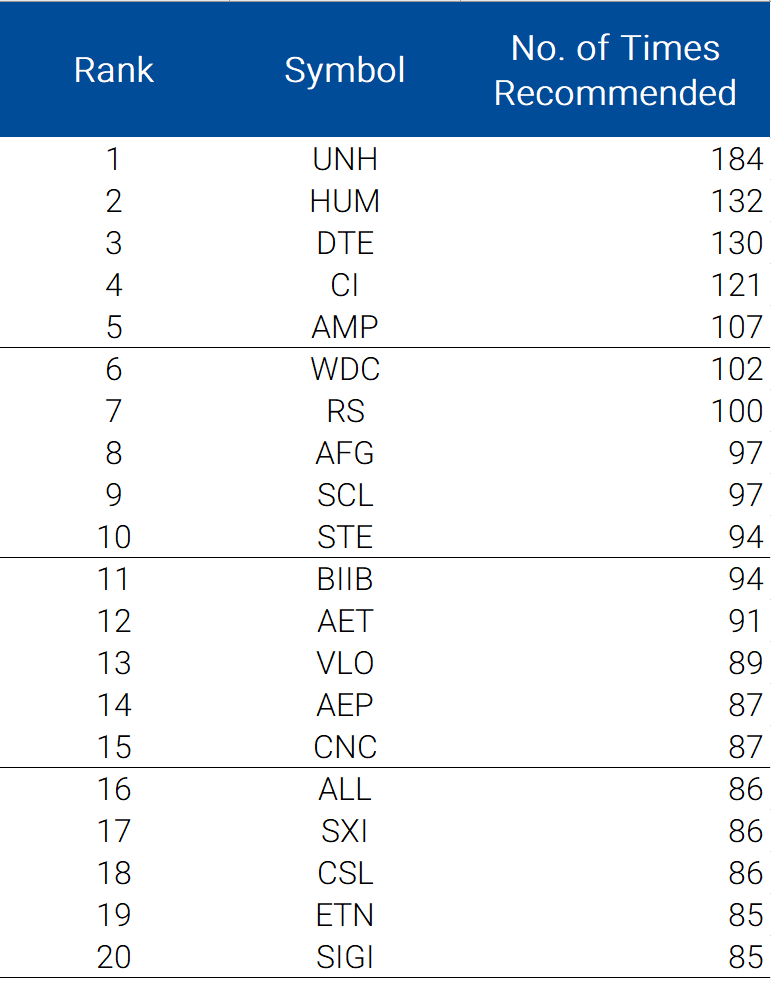
5. I then created a table showing each stock and how many times each stock was recommended. Below is a list of the Top 20 most recommended stocks.

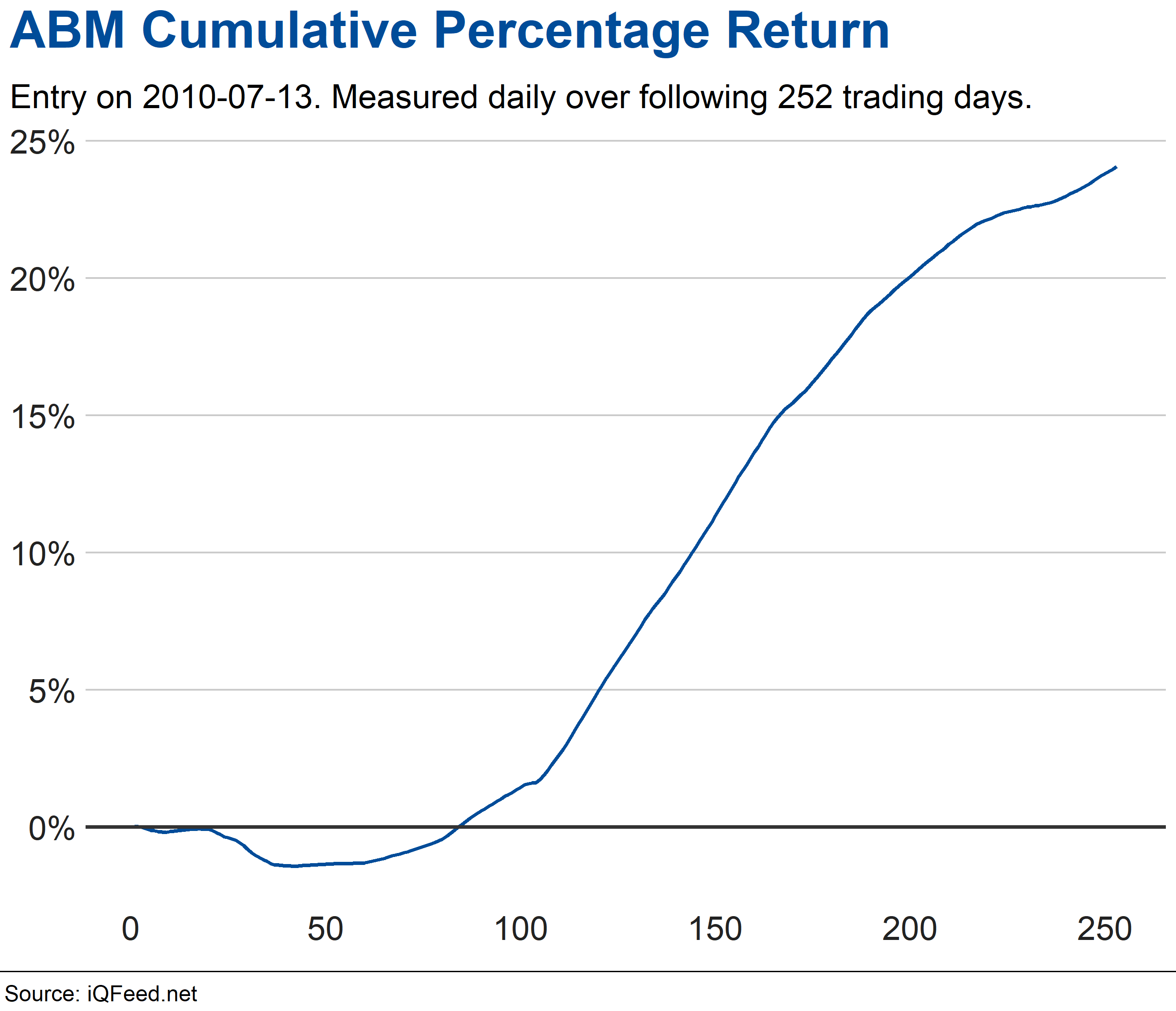
1. I then separated the cumulative daily percent return for EACH STOCK (rather than by recommendation date, as in Step 4 above). This return was measured from the Entry Date. This allowed me to analyze the cumulative return of each stock recommendation from 1 to nDays. For example, ABM was recommended 49 times during the time period tested. The first time was on 2010-07-13, and on that date it opened at 21.56. Below is the cumulative returns for the following 252 trading days. As you can see, it performed rather well.

1. I also separated the daily percent return (day over day returns) for each stock from the date of the recommendation. This helped in evaluating the day-to-day performance of each recommendation.

Results

Initially, it was difficult to measure the performance of the system against the S&P1500 benchmark. Comparing the cumulative performance against a benchmark proved futile. However, it was easier comparing the system on a day-to-day basis versus the benchmark. I attempted to annualize the 30/90/180 day exit performance so as to compare that against the historical annualized performance of the S&P Composite 1500. Additionally, I was only able to obtain information on the S&P Composite 1500 dating back to August 31, 2009. For that reason, relevant benchmark comparisons will ignore any recommendations prior to this date.

Exit After 30 Calendar Days From Entry Date

Cumulative Percent Return with 30 Day Exit

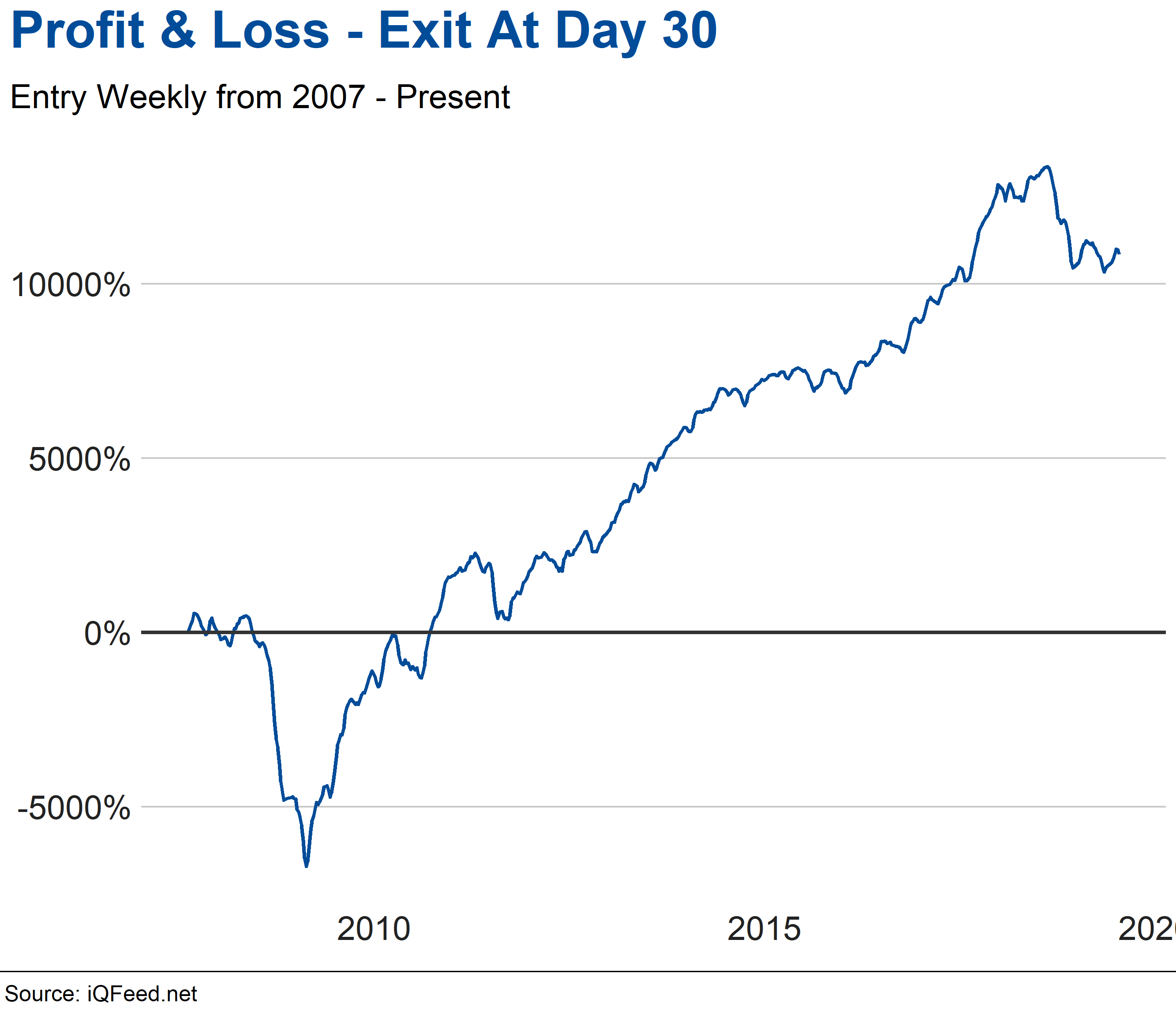
Exiting at 30 days after recommendation provided an average return of .67%, a winning percentage of 56.12%, a profit factor (Average Win/Average Loss) of -.95 and a cumulative return of 10,838%.

Benchmark Comparison with 30 Day Exit

Since August 31, 2009, the 30 day exit strategy provided an annualized return of 12.58% with annualized volatility (risk) of 28.4% for a Sharpe Ratio of 0.44.

This compares unfavorably versus the S&P Composite 1500 - see the table below.

	Annualized Return (%)	Annualized Risk (%)	Sharpe Ratio
30 Day Strategy	12.58	28.49	0.44
Benchmark	13.42	12.77	1.05

Note: see this link for calculating Annualized Standard Deviation of Monthly / Quarterly Return.

Cumulative Percent Return with 90 Day Exit

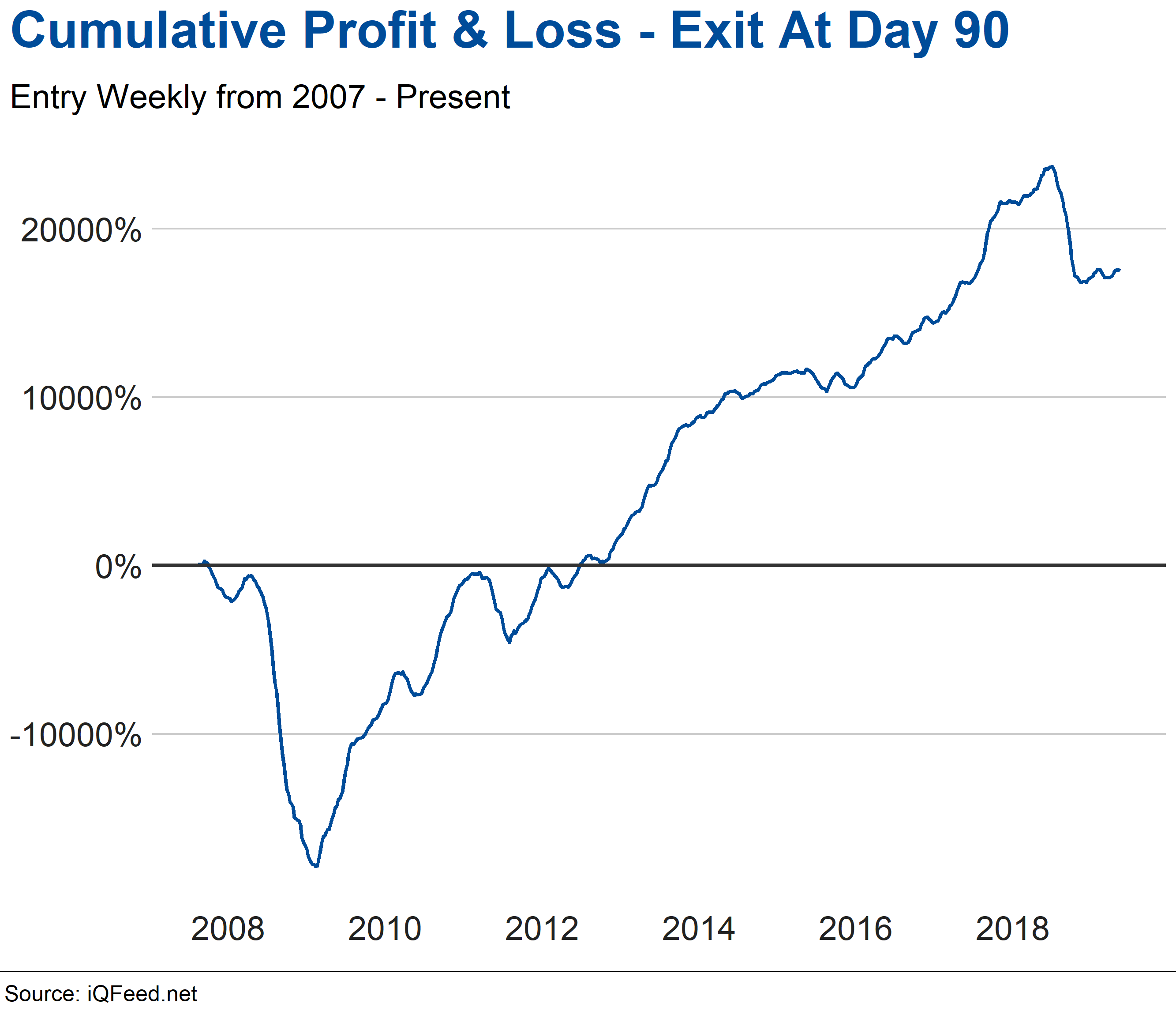
Exiting at 90 days after recommendation provided an average return of 1.2%, a winning percentage of 55.7%, a profit factor (Average Win/Average Loss) of -.97 and a cumulative return of 17,646%.

Benchmark Comparison with 90 Day Exit

Since August 31, 2009, the 90 day exit strategy provided an annualized return of 9.8% with annualized volatility (risk) of 28.31% for a Sharpe Ratio of .35.

This is not as favorable to the benchmark - see table below.

	Annualized Return (%)	Annualized Risk (%)	Sharpe Ratio
90 Day Strategy	9.8	28.31	0.35
Benchmark	13.42	12.77	1.05

Cumulative Percent Return with 180 Day Exit

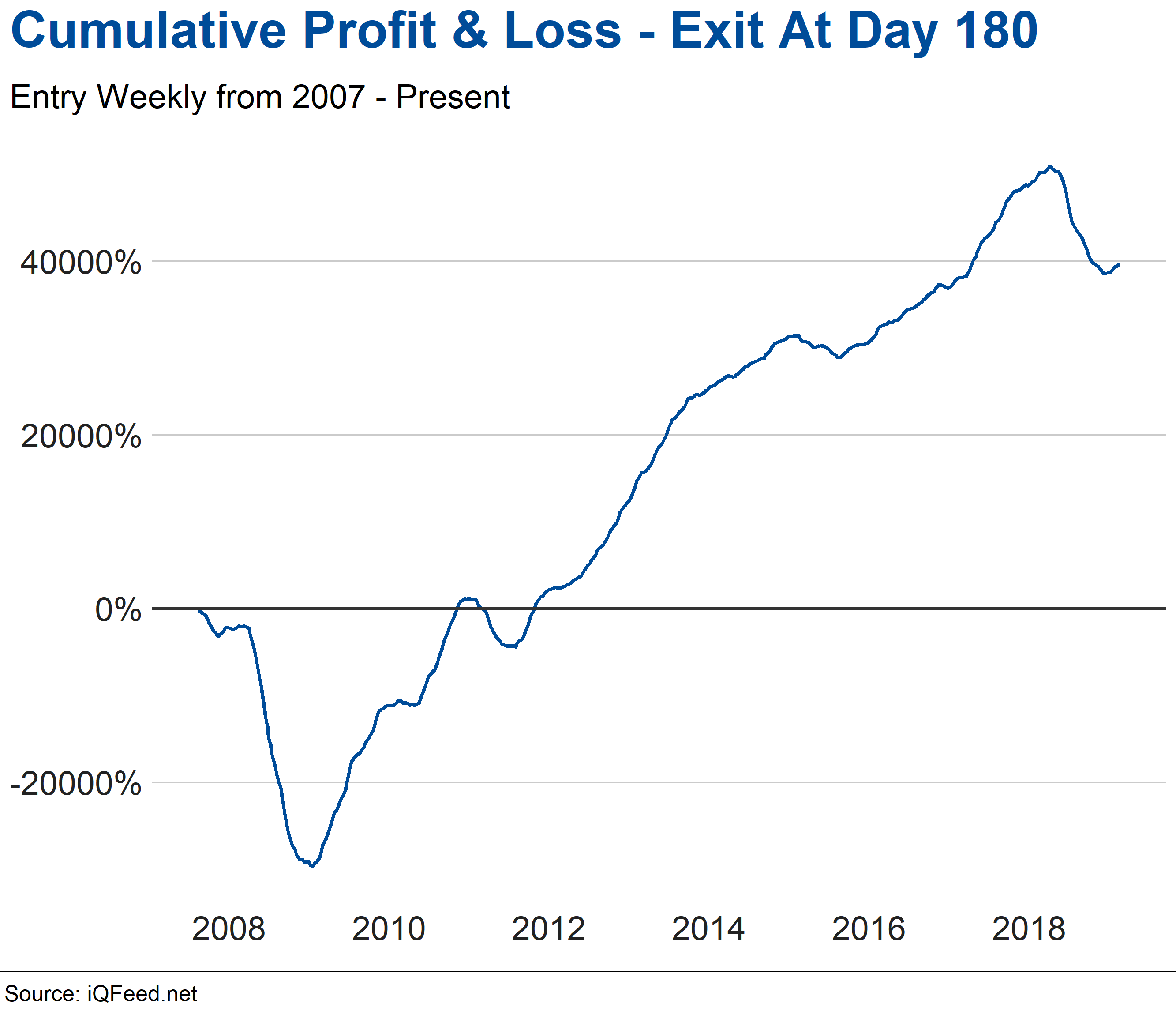
Exiting at 180 days after recommendation provided an average return of 2.8%, a winning percentage of 56.8%, a profit factor (Average Win/Average Loss) of -1.05 and a cumulative return of 39,545%.

Benchmark Comparison with 180 Day Exit

Since August 31, 2009, the 180 day exit strategy provided an annualized return of 10.17% with annualized volatility (risk) of 28.4% for a Sharpe Ratio of .35.

This is not as favorable to the benchmark - see table below.

	Annualized Return (%)	Annualized Risk (%)	Sharpe Ratio
180 Day Strategy	10.17	28.4	0.35
Benchmark	13.42	12.77	1.05

Cumulative Percent Return with 365 Day Exit

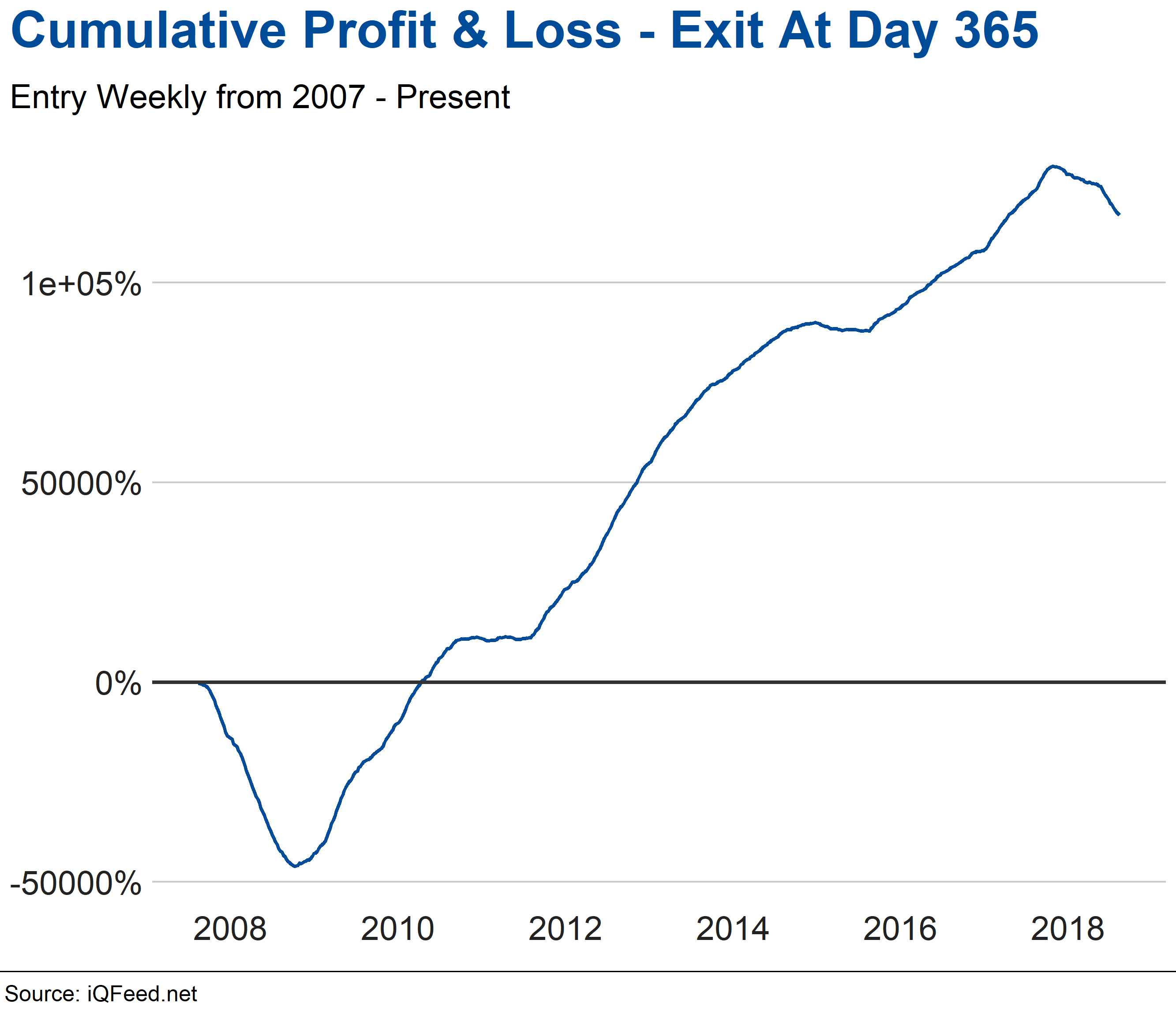
Exiting at 365 days after recommendation provided an average return of 8.3%, a winning percentage of 61.3%, a profit factor (Average Win/Average Loss) of -1.24 and a cumulative return of 116,981%.

Benchmark Comparison with 365 Day Exit

Since August 31, 2009, the 365 day exit strategy provided an annualized return of 11.9% with annualized volatility (risk) of 29.45% for a Sharpe Ratio of .40.

This is not as favorable to the benchmark - see table below.

	Annualized Return (%)	Annualized Risk (%)	Sharpe Ratio
365 Day Strategy	11.9	29.45	.406
Benchmark	13.42	12.77	1.05

Conclusion

Over each time period, the strategy had a lower risk-adjusted return as compared to the S&P Composite 1500 benchmark. However, over the short-term, the Top 40 Bespoke Stock Scores significantly outperformed the benchmark on a pure, risk-unadjusted annualized return basis. For instance, exiting at 10 days provided a 17.24% annualized return, exceeding the benchmark by more than 4 points.

Notes & Additional Research

1. See this excellent blog post on evaluating trading strategies in R. How to Measure the Performance of a Trading Strategy. The author also includes a link to the R Code here: 1.005 Measuring Performance.R.

2. The graphs on this report were created using the BBC Visual and Data Journalism cookbook for R graphics. You can find all of the R code to recreate the BBC style graphics at the BBC Github Repository.

3. S&P 1500 historical performance was obtained from the S&P Composite 1500 Page.

4. “Annualized Return is the constant annual return applied to each period in arrays that would result in the actual compounded return over that range. An Annualized Return is a special case of a Geometric Average Return where the time periods are expressed in terms of years.” See CRSP Calculations.