Monte Carlo Benchmarking for Trading Systems in R

Introduction

Part of the challenge of backtesting is coming up with a repeatable framework to compare trading systems. In this example, I will use Monte Carlo simulation in R as a way to measure whether or not a particular trading system is better than pure chance.

Overview

• Introduction
• Research
  • Monte-Carlo Methods
  • Coin Flip Systems and Random Returns
  • Monte Carlo Simulations of the Coin Flip System
  • A (Slightly) More Complicated Trading System: Bollinger Band Strategy
  • Monte Carlo Simulation of the Bollinger Band Strategy
• Conclusions
• Research and Notes

Research

Monte-Carlo Methods

“Monte Carlo methods (or Monte Carlo experiments) are a broad class of computational algorithms that rely on repeated random sampling to obtain numerical results; typically one runs simulations many times over in order to obtain the distribution of an unknown probabilistic entity. The name comes from the resemblance of the technique to the act of playing and recording results in a real gambling casino. “ [Wikipedia.(http://en.wikipedia.org/wiki/Monte_Carlo_methods)

A trading system is nothing more than a collection of rules to enter a long (+1), short (-1) or neutral position (0) in a financial instrument. “If the rule that determines the position to take each time a trading opportunity arises is an intelligent rule, the sum of the obtained returns will be larger than the sum that could be expected from a rule that assigns positions randomly.” See Monte-Carlo Evaluation of Trading Systems.

At its core, Monte-Carlo simulation is a method that: (1) models a problem, (2) randomly simulates the outcome a large number of times, and (3) applies statistical analysis to the output to evaluate the model’s probabilistic characteristics. You can then compare the Monte-Carlo simulation to the trading system results to determine if they were obtained by luck or through a real trading edge.

Whether a trading system has an edge or has attained its returns through randomness can be tested (relatively) easy in R. In statistical terms, a Monte-Carlo simulation tests the null hypothesis that the pairing of long/short/neutral positions with raw returns is random. See Monte-Carlo Evaluation of Trading Systems.

A Null Hypothesis is the hypothesis that sample observations result purely from chance. The Alternative Hypothesis “is the hypothesis that sample observations are influenced by some non-random cause.””

In trading terms, we are trying to determine whether the system is intelligently designed to produce superior returns (our Alternative Hypothesis) as compared with a random benchmark (our Null Hypothesis).

“A significance test is performed by assuming the so-called null hypothesis, which asserts that the measured effect occurs due to sampling error alone. If the null hypothesis is rejected, it’s concluded that the measured effect is due to something more than just sampling error (i.e., it’s significant). To determine whether the null hypothesis should be rejected, a significance or confidence level is chosen. For example, a significance level of 0.05 represents a confidence level of 95%. The so-called p-value is the probability of obtaining the measured statistic if the null hypothesis is true. The smaller the p-value the better. If the p-value is less than the significance level (e.g., p < 0.05), then the null hypothesis is rejected, and the test statistic is deemed to be statistically significant.” See Is That Back-Test Result Good or Just Lucky?

Coin Flip Systems and Random Returns

A completely random trading system enters and exits the market without regard to the past, current or the future or any outside indicators.

Assume we create a trading system that enters and exits an ETF at the end of each trading day based on the outcome of a flip of a coin. We assume a fair coin and that a heads (a “1”) means we are long the market and a tails (a “-1”) means we are short the market. We repeat this daily - going long or going short each day. See My Old Blog For More Information on This.

We have two input time series for the trading system: (1) the Rule Position which is the coin flip entry rule be long or short; and (2) the Market or Raw Return which is the daily return of the financial instrument. SeeMonte Carlo Permutation: Test your Back-Tests

Our Null Hypothesis is that half of the flips will be heads and half of the flips will be tails, i.e., we will be long half the time and short half the time. Stated otherwise, the returns of the Coin Flip System are a randomly correlated to Market or Raw returns. The Alternative Hypothesis is that the Coin Flip System is a sample from a profitable population, and that the Rule Position is correlated to market returns.

Below is the code to simulate coin flips with a 50% probability of coming up with either heads or tails. See Simulating a Coin Flip in R. Note that we are flipping the coin a number of times equal to the number of trading days for QQQ.

sample.space <- c(-1,1)
theta <- 0.5  ##this is a fair coin
N <- length(Close[[1]]) ## match number of flips to total trading days

flips <- sample(sample.space,
                size = N,
                replace = TRUE,
                prob = c(theta, 1 - theta))

Next, we apply the “coin flip” outcome (which is our Rule Position) to the daily returns of QQQ (which is our Raw or Market Return) and then plot the cumulative returns during the trading period.

Coin.Flip.System <-
  all.stock.data[[1]] %>%
    mutate(
    daily.return = ifelse(row_number() == 1, 0, close / lag(close, 1) - 1),

    signal.return = daily.return *  flips,

    cum.return = cumprod(1+signal.return) - 1)

Using our coin-flip trading system, let’s apply it to the daily returns of the Nasdaq-100 based ETF QQQ. The chart below shows the cumulative daily returns of the Coin Flip System.

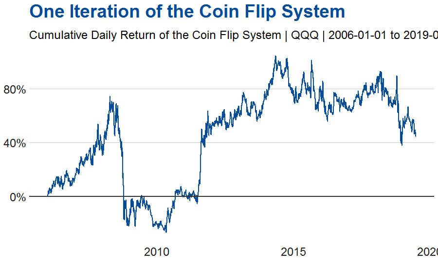
This is only one iteration/run of our trading system. What if we want to know all of the possible paths the ETF could take?

Monte Carlo Simulations of the Coin Flip System

Solve for the standard deviation and average return of the Coin Flip System, and then find the average daily return and the average standard deviation of these daily returns of the system.

MC.Coin.Flip.System <-
  all.stock.data[[1]] %>%
    mutate(
    daily.return = ifelse(row_number() == 1, 0, close / lag(close, 1) - 1),

    signal.return = daily.return *  flips,

    cum.return = cumprod(1+signal.return) - 1,

    sd = runSD(daily.return, n = 252)*sqrt(252),

    sd.2 = runSD(daily.return))

MC.Coin.Flip.System.sd <- mean(MC.Coin.Flip.System$sd.2, na.rm = T)

MC.Coin.Flip.System.avg <- mean(MC.Coin.Flip.System$daily.return, na.rm = T)

Next, we create a function that projects a normal distribution of the daily returns of the Coin Flip System. We apply those different paths to the closing value of QQQ from the first date we evaluate the ETF (here it is 2016-01-03) to the final closing price. Much of this code is taken from the post Monte Carlo Simulations in R on the incredible Count Bayesie Blog.

MC.Coin.Flip.System.generate.path <- function(){

  MC.Coin.Flip.System.days <- length(Close[[1]])

  MC.Coin.Flip.System.changes <-

  rnorm(length(Close[[1]]),mean=(1+MC.Coin.Flip.System.avg),sd=MC.Coin.Flip.System.sd)

  MC.Coin.Flip.System.sample.path <- cumprod(c(Open[[1]][[1]],MC.Coin.Flip.System.changes))

  MC.Coin.Flip.System.closing.price <- MC.Coin.Flip.System.sample.path[days+1]

  return(MC.Coin.Flip.System.closing.price/Open[[1]][[1]]-1)
}

Now replicate the Coin Flip System path 100,000 times and then solve for the median value of the stock and the upper and lower 95th percentiles.

MC.Coin.Flip.System.runs <- 100000
MC.Coin.Flip.System.closing <- replicate(runs,MC.Coin.Flip.System.generate.path())

median(MC.Coin.Flip.System.closing)
quantile(MC.Coin.Flip.System.closing,probs = c(0.05,0.95))

Repeat the Monte Carlo Simulation process for the underlying ETF by solving for the average daily return and standard deviation then simulate 100,000 different paths QQQ could have taken.

	Coin Flip System Return (%)	ETF Return (%)
Median	385%	386%
Mean	498%	499%
95th Percentile	1307%	1310%
5th Percentile	66.3%	66.5%

The similarities between the Coin Flip System and the market returns for the ETF are virtually the same. Why? Mainly because of the similarities between the average and standard deviation of the Coin Flip System and the ETF itself. Sine the Coin Flip System is either long or short the underlying ETF, it was highly probable that the system and the ETF would have the same statistical characteristics.

The chart below models one of the simulated returns for our Coin Flip System (in red) and one of the simulated returns for the underlying QQQ ETF (in blue).

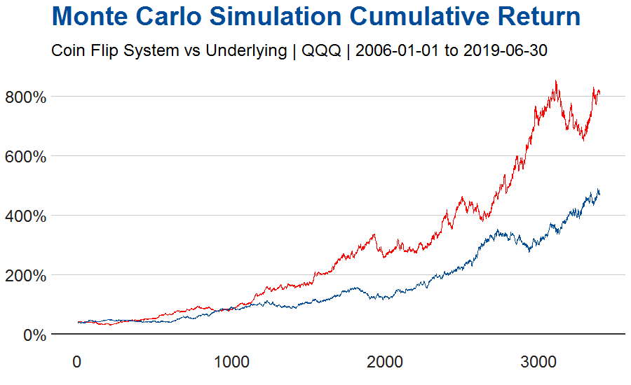
Comparing the median and confidence intervals of the Coin Flip System vs the random entry into the ETF, we cannot reject the Null Hypothesis that the Coin Flip System results were purely by chance. From a practical standpoint, we knew this going in because the entry and exit is purely random being entirely based on an equal (50/50 chance of either being long or short.

But what if you can’t use the “eye test” for evaluating whether or not the results were random?

“The p-value of the original back-testing sample can then be computed (it is equal to the fraction of random rule returns equal or greater to the back-tested rule return).” Source. In this example, the average ETF cumulative return is 499%. The Null Hypothesis is that the cumulative return of the Coin Flip System in excess of the average ETF cumulative return are random.

Calculate the t-test distribution and the p-value in excess of the average return.

t <- (mean(MC.Coin.Flip.System.closing,na.rm = T)-mean(mc.closing))/(sd(MC.Coin.Flip.System.closing)/sqrt(length(MC.Coin.Flip.System.closing)))

p <- 2*pt(-abs(t),df=length(MC.Coin.Flip.System.closing)-1)

This results in a p-value for the Coin Flip System of 0.71. This is well short of the statistical significance threshhold of 0.05 for a p-value (the null hypothesis would be rejected for any p-value less than 0.05). We cannot reject the null hypothesis that the Coin Flip System cumulative return is not by chance.

Although it is likely self evident, you would not want to trade the Coin Flip System even if you got a result showing that the system had a very positive return. If you look at the chart above it appears that the Coin Flip System significantly outperforms being long the ETF. This is a fluke - a false trading strategy that, in reality, was just one path the strategy could have taken. I will discuss false trading strategies in a separate post.

A (Slightly) More Complicated Trading System: Bollinger Band Strategy

Bollinger Bands measure the historical volatility of an instrument above and below a simple moving average. A simple Bollinger Bands system is a mean reverting strategy that would enter long when price crossed over the lower band and enter short when price crosses the upper band. This simple strategy is always exposed to the market; it is never flat.

Although the TTR Package in R supports the use of Bollinger Bands, I will construct them from scratch.

First, assign the length for the simple moving average (the middle band) and the average for the upper and lower bands. Here, I use the traditional SMA setting of 20 periods.

Assign the displacement for the upper and lower bands. I set the upper and lower bands 2 standard deviations above and below the simple moving average.

Using the OHLC from the ETF, set the rolling standard deviations and calculate the middle, upper and lower bands. Our signal will enter long (+1) if the close is less than lower band and enter short (-1) if the close is greater than the upper band. Note that denoting a short as “-1” and then multiplying that by the daily return of the instrument, gives us the correct return. For example, if the ETF is -1% for the day amd we are short, the end result is a gain of 1%.

BBand.Avg.Length <- 20

BBand.SD <- 2

BBand.System <-
  all.stock.data[[1]] %>%

    select(date,open,high,low,close) %>%

    mutate(
      daily.return = ifelse(row_number() == 1, 0, close / lag(close, 1) - 1),

      cum.daily.return =
        (cumprod(1+daily.return)-1)*100,

      sd = runSD(close),

      middle.band = ifelse(row_number() >= BBand.Avg.Length,  rollmean(close, k = BBand.Avg.Length, fill = NA), 0),

      upper.band = ifelse(row_number() >= BBand.Avg.Length,  rollmean(close, k = BBand.Avg.Length, fill = NA) + (BBand.SD * rollmean(sd, k = BBand.Avg.Length, fill = NA, 0)),0),

      lower.band = ifelse(row_number() >= BBand.Avg.Length,  rollmean(close, k = BBand.Avg.Length, fill = NA) - (BBand.SD * rollmean(sd, k = BBand.Avg.Length, fill = NA, 0)),0),

      signal =
        ifelse(close < lower.band,1,
          ifelse(close > upper.band,-1,NA)),

      signal.2 =
        na.locf(signal),

      signal.return = daily.return *  signal.2,

      cum.signal.return = (cumprod(1+signal.return) - 1)*100)

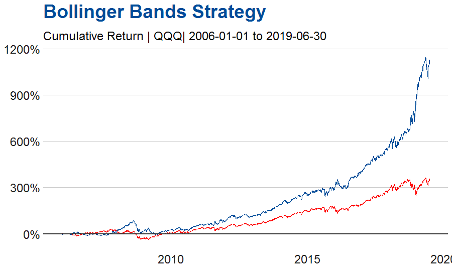
The chart below shows the comparison of the cumulative daily returns of QQQ (in red) vs the Bollinger Bands strategy (in blue).

Monte Carlo Simulation of the Bollinger Band Strategy

Analyzing the Bollinger Band Strategy as compared to being long the QQQ ETF, and assuming a 13.5 year holding period from 2006-01-01 to 2019-06-30, the results are as follows:

	BBands Strategy	QQQ ETF
Average Daily Return	0.08%	.05%
Average Standard Deviation	1.13%	1.47%
Maximum Drawdown	-444.79%	-324.67%
Average Sharpe Ratio	1.14	0.73
Cumulative Return	1114.30%	352.04%
Annualized Return	20.30%	11.82%

Using the same Monte Carlo Analysis above on the Bollinger Band Strategy and utilizing 100,000 runs, the median cumulative return for the Bollinger Bands strategy is 1195%, with a 95% confidence return between 340% to 3722%.

For the ETF, Monte Carlo Analysis returns a median cumulative return of 382%, average cumulative return of 499%, with a 95% confidence return between 62% to 1325%.

Solving for the t-distribution of the excess returns of the Bollinger Band Strategy versus the ETF yields 267.90. This yields an extremely small p-value; it is essentially zero, which means we can reject the null hypothesis. In other words, it is likely that the Bollinger Band strategy provides an edge. This is not a recommendation to trade this strategy. More testing is needed to determine if this strategy is viable.

Conclusions

Monte Carlo methods are a good tool to have to determine if a given trading strategy is due to chance or (rather) from a statistically significant edge. In future posts, I will examine other methods to determine if the strategy is tradeable. These include Bootstrapping, Jacknife, Permutation Testing and Cross-Validation.

Research and Notes

1. For an excellent read on how to construct your own “synthetic” security, check out Coin Tosses and Stock Price Charts by Timothy R. Mayes, Ph.D.

2. A Brief Overview of Bollinger Bands. Stock Charts - Bollinger Bands.

3. An Overview of Using Moving Averages in R. UC Business Analytics R Programming Guide - Moving Averages.

4. Pitfalls of Using Monte Carlo Analysis. System Trader Success - Fooled by Monte Carlo Analysis.

5. Trading System Evaluation. Evaluating Trading Systems By John Ehlers and Ric Way.

6. An incredible overview of Monte Carlo Analysis Permutation Usage when evaluating trading systems. Evidence Based Technical Analysis - Monte Carlo Permutation Evaluation of Trading Systems.

7. Table of contents generator for MarkDown.

8. Coin Flips, Risk to Reward Profile and Creating Your Own Synthetic Security from my old blog Mind Right Trading.

9. An interesting paper on Evaluating Trading Strategies. The authors review several methods for calculating a t-statistic formula using the Sharpe Ratio of the trading strategy. This is calculated by multiplying the Sharpe Ratio times the square root of the number of years the strategy traded. For instance, a t-statistic of 2.91 means that the observed profitability is three standard deviations from the null hypothesis of zero profitability. The paper expands on this formula, covering the problems of multi-testing trading strategies by using the family-wise error rate (FWER) and the false discovery rate (FDR).

10. 2 great articles on the specifics of Monte Carlo Permutation when evaluating trading strategies: (1) Monte Carlo Permutation: Test your Back-Tests; and (2) Is That Back-Test Result Good or Just Lucky?

11. An intense and lengthy overview on StackExchange of Resampling / simulation methods: monte carlo, bootstrapping, jackknifing, cross-validation, randomization tests, and permutation tests.

12. Chapter 10 of the very helpful R Tutorial shows several ways of calculating a p-value.