Problems with Backtesting Signals
>Overview
A signal is triggered based on the result of a function or indicator. Generally, a signal is indicated at some point during the period of time-series data. For stocks, options and other financial options that is generally at the Open, High, Low or Close (“OHLC”) of a bar. For tick-based data, the signal triggers at the moment the tick (or trade) is registered. I address the difference between a signal and a position and offer some ways to deal with each.
Signal vs Position
For my purposes, a signal only indicates the existence of a certain condition (ie, the RSI indicator is greater than 70 or the 50 period SMA has crossed over the 200 period SMA), and that the condition indicates the direction and entry and/or exit value of a trade (ie, -1 for sell to open (short)/sell to close and +1 for buy to open (long)/buy to cover). A position is the actual application of the signal to the time-series data. This may seem inconsequential, but in reality it has significant implications.
Separating the signal and the position recognizes that both can’t occur at the same time. For example, you can’t have a SMA crossover indicating a long position (+1) occur at the same time you actually buy to open. The signal occurs at some time (“time.1”) before the position can be initiated at a later time (“time.2”).
Whether the time difference between time.1 (signal) and time.2 (position) is large or small depends on various factors.
How often is the signal evaluated? For OHLC data, if the signal only evaluates at the open of a bar, then the position can only be initiated at some point after the open - likely at the next H, L or C.
How long is the period? Daily bars will obviously have a longer time between signal and position than 1-minute or tick data. This leaves more time between each.
How liquid is the data and what assumptions are being made about slippage? Slippage is a projected amount that the position will vary from the intended time period to enter or exit a position. Among other reasons, it can be caused by lack of liquidity, volume, instrument turnover, and broad bid-ask spreads.
For example, assume a strategy fires a long (+1) signal at the open of a bar and the position is initiated at the close of the bar. Slippage would work against the position; an amount would be deducted from the close to simulate the possibility of an entry that is worse that what was expected. This is a conservative approach since you never want to assume that you will get a better fill than the most recent price. The opposite is true for a short (-1) position. A worse position is simulated by adding to the assumed entry.
Avoiding Look-Ahead Bias
If a signal fires at time.1, then the position must occur at some point after the signal at time.2. The position is either on the next tick or following the OHLC. This presents a challenge when backtesting a strategy. Often I see strategies that will both trigger a signal and enter on the same period. For example, a moving average crossover signals at 9:50 a.m. at the open of the bar and a long entry simultaneously occurs at the same open. This is called look-ahead bias and can return overly favorable performance analytics. The Capital Spectator explains look-ahead bias:
Take a strategy that issues a “sell” signal when price falls below an x-day moving average and a “buy” when price rises above that average. Let’s also assume that we’re using end-of-day closing prices. You test the strategy and discover that it delivers a strong performance through time. But you forget one small item: the end-of-day signals aren’t available until after the market closes. In other words, calculating returns for a real-world version of the strategy requires using lagged “buy” and “sell” signals.
For OHLC bars, you have two options to avoid look-ahead bias:
1. use a lagged signal for the position, or
2. calculate an average to impute what the entry position would be.
A lagged signal will generally always be your most accurate option, but there are some cases where imputing a value can be more conservative.
<a name”lagged-signals-for-positions”>Lagged signals for positions
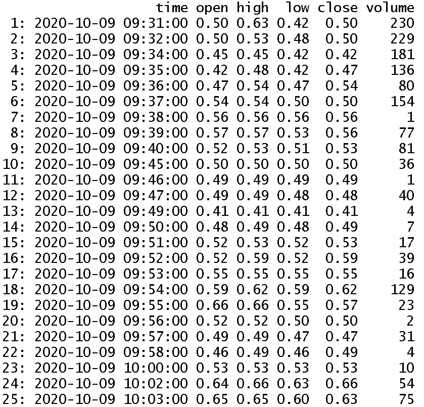
Assume you have the following OHLC data for a 1-minute bar:
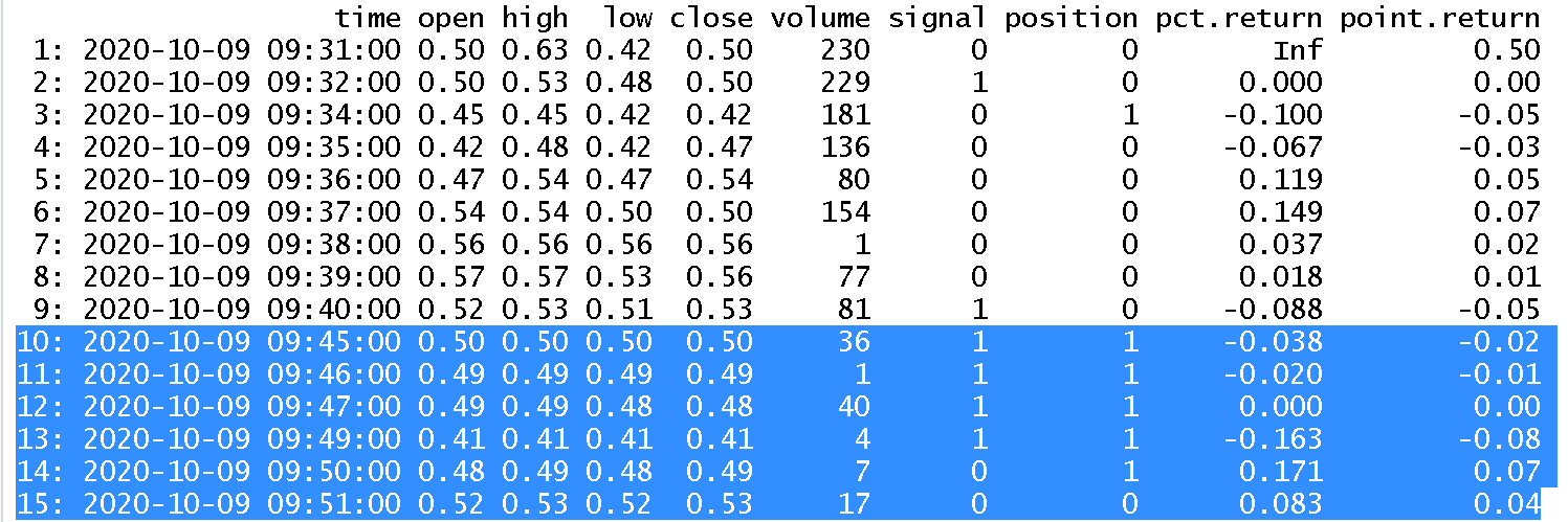
You have a strategy that has a long signal based on some unknown function. I added the signal column to the dataframe:
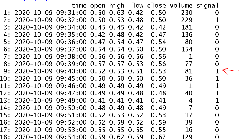
The poorly-drawn red arrow indicates a long signal at 09:40:00 am. You can’t go long at that time since the signal fired then. You can only enter long at some point after that signal.
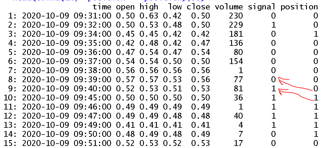
I added a column using the lag() function that essentially looks back n number of periods from each period. At 09:40:00 am, it will look back 1 period to 09:39:00 am and see if a position should be initiated. I set the default value to zero, which tells the command to insert a 0 for the first value (since there is no period prior to it) rather than an NA value.
position = lag(signal, n = 1, default = 0)
position Value: Percentages and Points
Once the position is established, you can decide exactly where to enter or if slippage should be added. For example, if you enter the position at 09:45:00 am, should it be at the O, H, L or C of the 09:45:00 am bar? Are you measuring percentage return or total amount returned?
This is where additional errors can be made, if you are not careful. The goal of the backtest is to find the value of your account after the signal and position have been initiated and completed. In other words, you want to find the difference in points and/or percent of the exit minus the entry. Assume the strategy enters and exits at the open for this example.
The signal fired +1 at 09:40:00 am, the position went long at 09:45:00 am, the signal stayed at +1 until 09:50:00 am when it went flat (0), meaning the position went flat 1 period later at 09:51:00 am. At the entry at bar 10 (09:45:00 am) the open was 0.50 until the exit at bar 15 (09:51:00 am) where the open is 0.52 (I will now go retire on my 0.02 gain, sucka).
The normal way to solve for returns is to add a column showing the percent or point returns from the open of the current bar back to the open of the prior bar. For example, the percent return at bar 9 is the open of bar 9 minus the open of bar 8 minus 1 (which is 0.53/0.56 - 1 = -8.7%). I added a column with percent returns and point returns:
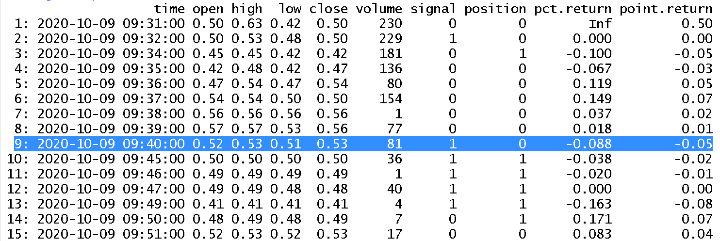
Point returns are similar. At bar 9, the change in value from bar 8 was -0.02 points.
The issue with using the 1-bar look back point and percent returns is that it tells us nothing about what is happening from the position entry at the open on bar 10 to the position exit at the open on bar 15.
The sum of the point.return from bar 10 to bar 15 are
> -.02 + -.01 + 0 + -.08 + 0 + 0
[1] -0.11
But wait, didn’t we show the difference between the exit at bar 15 and the entry at bar 10 was a 0.02 gain? That’s a lot different than -0.11!
The reason is that the point.return column from bar 10 to bar 15 is actually showing the return from the open at bar 9 to the open at bar 15. This is not what we want!
This can be solved by using a function again to calculate the correct returns. For this example, that means shifting the returns forward using the lead() function. This acts the same as lag() but in reverse. At each bar, it looks forward to the next value and returns it.
pct.return.lead = lead(open, n = 1, default = 0)/open - 1
pt.return.lead = lead(open, n = 1, default = 0) - open
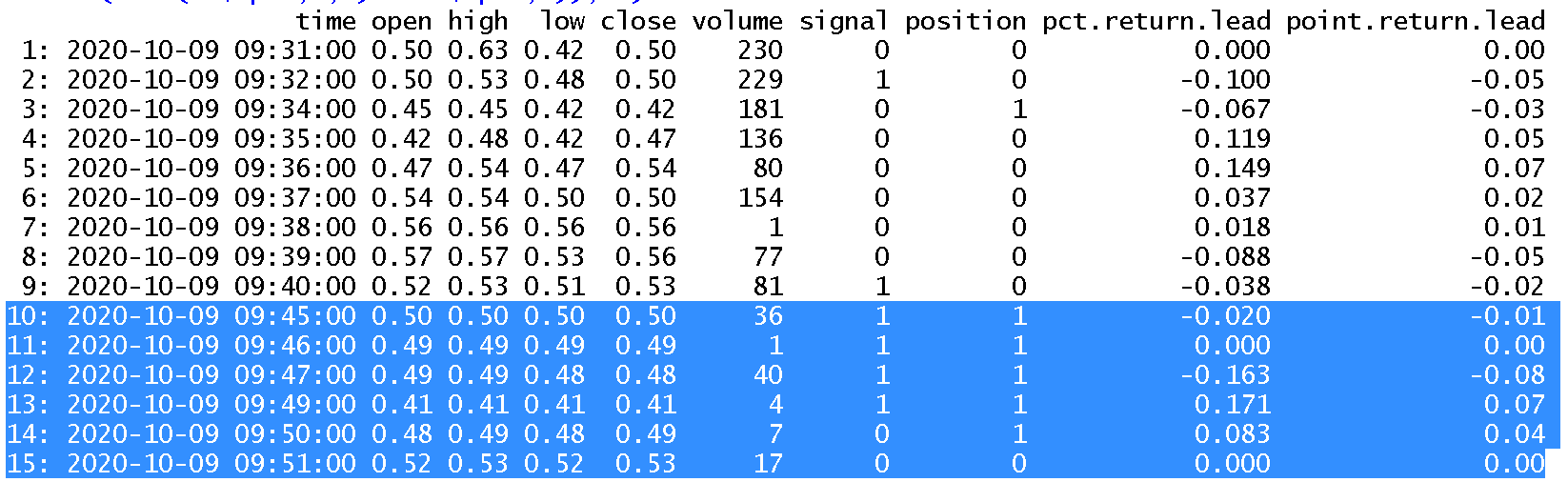
Now adding the point.return.lead from row 10 to row 15 gives us the correct answer:
> -.01 + 0 + -.08 + .07 + .04
[1] 0.02
In other words, lag() the signal to get the correct position and lead() the returns to get the correct future returns.
<a name”impute-a-value-for-the-position”>Impute a Value for the position
This is not my favorite way to find a value for the position, and I will only briefly discuss it, but you can use an imputed value. Generally, this is an average of the H and L of the position bar, a linear regression based on a relative look-back period or some other function or indicator. Unless absolutely necessary, why implement fake data when actual data is available? Most times any simulation can be modified with slippage.