Random Everything - Testing What is Really Important
Overview
I often hear that the “best traders” can take a random entry and profit by simply managing the trade and applying appropriate account management principles. Through Monte Carlo analysis and other statistical tests applied to the random walk hypothesis, synthetic and actual stock data for stocks across the S&P 500, I examine whether this is true or not for a limited number of post-entry management techniques, including random exits, profit-targets, stop-losses and trailing-stops.
TOC
- Research: Randomness Be Thy Name
- Coin-Flip Stock Tests
- Actual Stock Data Tests
- Test 1: Random Entry/Random Exit for Actual Stock Data
- Test 2: Random Entry/Stop-Loss or Profit Target Exit for Actual Stock Data
- Test 3: Random Entry/Trailing Stop (%) Exit for Actual Stock Data
- Test 4: Random Entry/Trailing Stop (%) or Profit-Target(%) Exit for Actual Stock Data
- What now, Donny? A Summary of Actual Data Testing
- Other Tests and Research
- Conclusion
- Notes & Research
Research: Randomness Be Thy Name
Types of Entries and Exits
Entering a trade (either by buying to open or selling short to open) or exiting a trade (selling to close or buying to cover to close) means that the trader is initiating a position in a financial instrument. For ease of reference, “entry” or “entering” a position will be used for buy to open or sell short to open, and “exit” or “exiting” will be used for sell to close or buy to cover.
To simplify, entries and exits can categorized as follows (Note: I am leaving a lot of entry and exit options out - this is not meant to be an exhaustive list):
Random
Example: buy to open/sell short to open at random and sell to close/buy to cover at random
Time Based
Example: buy to open/sell short to open at 09:30:00 a.m. and sell to close/buy to cover at 10:00:00 a.m.
The underlying “reason” for the time based entry or exit is inconsequential. Choosing to enter/exit a position at a given time might be based on a random signal, an indicator or for some other reason. Regardless, the time is what determines exit and entry.
Price Based (amt or % or indicator)
Example: buy to open at $249.
Volume Based (amt or % or indicator)
Example: sell short to open after 5M shares have traded. Buy to cover if SMA20 of volume crosses below 3.5M shares.
Stop or Stop-Limit ($ or % or indicator)
Example: buy to open/sell short to open at $248.50 stop when the stock is trading at $249.00. The counterpart is to sell to close/buy to cover at $248.50 when you are currenly long or short the stock and the stock is trading at $249. A stop could also be triggered based on an indicator i.e. buy to open stop $248.50 if SMA 50 greater than SMA 200.
For this research, a stop and a stop-limit order are the same since we are backtesting the strategy and (based on the data used) can’t distinguish a stop “buy at market” or a stop-limit “buy at x price or better.”
Profit Target ($ or % or indicator)
Example: sell to close if profit is equal to $1000.
Note that profit target must take into account the current position (or non-position)
Trailing Stop ($ or % or indicator)
Example: exit the position if the open of the next bar is below 1% of the cumulative maximum.
All of the categories above can all be combined together to create a trading strategy. Assuming this is true, that gives 3.556874e+14 possible combinations for just the buy side (and that doesn’t calculate the endless array of paramaters and indicators you could appy). However, some of these are clearly not useful, and for the sake of keeping things simple, I will look at the following:
- Random Entry/Random Exit
- Random Entry/Profit Target(%) Exit
- Random Entry/Trailing Stop(%) Exit
- Random Entry/Profit Target or Trailing Stop(%) Exit
A Non-Random Fight Over Randomness
“In probability theory, a random walk is a stochastic process in which the change in the random variable is uncorrelated with past changes. Hence the change in the random variable cannot be forecasted. For a random walk, there is no pattern to the changes in the random variable, as the existence of any pattern would mean that the changes can be forecasted.” Source
If you ever want to start a fight, try to go into a room full of financial advisors and tell them that you can predict the market. The random walk hypothesis states that stock prices are (you guessed it) random and that they cannot be predicted. Entire industries and careers are predicated on the fact that you can’t predict the market. The simplified theory is that any outperformance - Alpha or whatever you call it - is only by chance.
Conversely, their are also entire industries and careers that are based on the fact that the market is not random and can therefore be predicted by trends, patterrns and historical price and volume action.
Both sides have their proponents: “[p]assive investments such as index funds and exchange-traded funds control about 60% of the equity assets, while quantitative funds, those which rely on trend-following models instead of fundamental research from humans, now account for 20% of the market share…” Source
For a short list of interesting articles on the topic, check out the Notes and Research Section at the end of this post.
Which side is right? Who cares, really. The key is you need to decide for yourself, and what better way to do that than some good ol’ fashioned statistical and Monte Carlo analysis.
And what if whether or not the stock market is random or not is the wrong answer to be asking? The sole aim of a trader is to extract as much money from the market as his/her account will allow (I’ll add that such extraction should be in an “ethical” manner but you define that term and make that decision for yourself). Why does it matter then if market movement is random or not? Something makes prices move and you should be agnostic about your belief in why it happens. Your only job is to profit off it. A short passage from Technical Analysis and Random Walks struck me as relevant:
“The term random has some unfortunate connotations. Random events are often believed to be in some sense “un-caused.” This belief is partly due to misleading comparisons that are sometimes drawn between stock price changes and the behavior of a roulette wheel. The problem is liable to be translated into a philosophical one, but there is nothing mystical or unnatural about the process that generates stock price changes. It is not governed by some frolicsome gremlin. The random movement of stock prices simply results from competition between a large number of skilled and acquisitive investors.”
Research Framework
First, I attempt to answer the question of whether or not an edge is required to be profitable.
I will test the 4 random entry and exit rules noted above on a few different “securities.” In essence, the random entry portion should (hypothetically) remove any “edge” from the equation, thereby allowing me to examine the effects of the post-entry management. I anticipate that the profit target, trailing stop and indicator may act as the “edge” that will ultimately be profitable.
The first “security” I test on is a “coin-flip” stock. The coin-flop stock is a synthetic security that has a normally distributed (ie, 50-50) chance of increasing or decreasing from one period to the next. To be somewhat consistent with the market, the coin-flip stock has a lognormal distribution of returns.
The second security will be actual daily stock data for the S&P 500. I will mass download the stock data, calculate the periodical returns and use Monte Carlo analysis to see whether the 4 random entry and exit rules are profitable.
Note that all tests will assume an equal amount of a hypothetical cash account is allocated to each test (ie, no compounding of the account).
Coin-Flip Stock
Assume for a second we have a purely “coin flip” stock. Whether the stock is positive or negative during a given period is 50-50. This is a Bernoulli distribution where one trial of an experiment yields either a success or a failure. I will ignore that a stock can remain flat (neither positive nor negative) from one period to the next. The distribution of returns for the “coin flip stock” is lognormal with a mean return of 0 and a standard deviation of 0.005.
set.seed(123)

# - normal distribution of positive or negative
p.sample.signal <- c(-1,1)
p.prob <- 0.5 #percent of times
p.periods <- 200 #number of periods

coin.flips <- sample(p.sample.signal,
                size = p.periods,
                replace = TRUE,
                prob = c(p.prob, 1 - p.prob))

# - lognormal distribution of returns
p.mean.log <- 0
p.sd.log <- .005
coin.returns <- rlnorm(n=p.periods,
                  meanlog = p.mean.log,
                  sdlog = p.sd.log)

# - position
coin.position <- (coin.returns-1)*coin.flips
Test 1: Random Entry/Random Exit for Coin-Flip Stock
Now I can build a function that finds the cumulative sum of the returns over a given number of periods. We can replicate this function hundreds of thousands of times.
fn.coin.flip <- function(
p.prob = 0.5,
p.periods = 200,
p.mean.log = 0,
p.sd.log = .005)
{
a <- sample(c(-1,1),p.periods,replace = TRUE, prob = c(p.prob, 1 - p.prob))
b <- rlnorm(p.periods, p.mean.log, p.sd.log)
c <- (b-1)*a
return(c)
}
fn.final.coin.flip <- function(){
a <- sum(fn.coin.flip(),na.rm = T)
return(a)
}
# - find the final value of the coin flip stock 100,000 times
mc.coin.flip <- replicate(100000, fn.final.coin.flip())
# - output a summary of the monte carlo simulation and a histogram
round(summary(mc.coin.flip),5)
# Min. 1st Qu. Median Mean 3rd Qu. Max.
# -0.30376 -0.04810 -0.00009 -0.00001 0.04829 0.29403
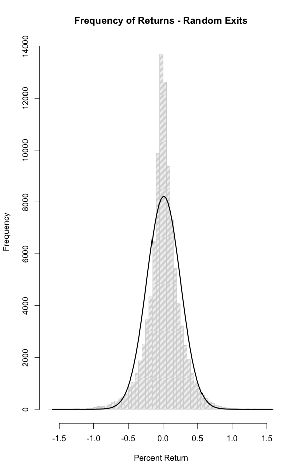
hist(mc.coin.flip,breaks = 100)
The results are what is to be expected: (1) 100,000 tests of the cumulative value of the returns after 200 periods averages 0, (2) the max return in all of the 100,000 tests is 29.4% and the minimum return is -30.4%, and (3) the histogram looks roughly normal.
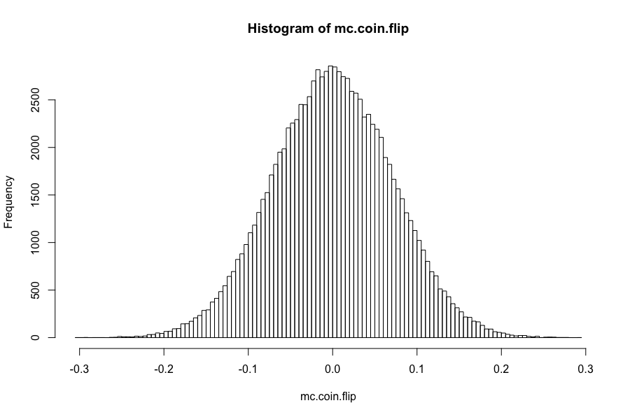
The conclusion? If we enter our coin flip stock at random and exit at random, over 100,000 returns, the average is zero. There is no edge in random entries and random exits for our coin-flip stock.
Test 2: Random Entry/Stop-Loss or Profit Target Exit for Coin-Flip Stock
The second test is to enter the coin-flip stock at random and then exit if either a profit target or a stop-loss is reached (whichever occurs first).
For the fixed stop-loss and profit target calculation, I will be using a modified function from the Systematic Investor Toolbox. Note: if you are an R trader, stop what you are doing and go directly to his blog. Do not pass go.
	fn.fixed.stop.fixed.pt <- function(weight, price, tstart, tend, pstop, pprofit) {
		index = tstart : tend
		if(weight > 0){
			temp = price[ index ] < (1 - pstop) * price[ tstart ]

      # profit target
			temp = temp | price[ index ] > (1 + pprofit) * price[ tstart ]

    } else{

			temp = price[ index ] > (1 + pstop) * price[ tstart ]

      # profit target
			temp = temp | price[ index ] < (1 - pprofit) * price[ tstart ]
    }
	}
Then put together a function that returns the simulated path of the coin-flip stock and the % return when either the stop-loss or the fixed profit-target fires. Notice that the default function reflects a 2:1 ratio of wins to losses.
fn.fixed.stop.fixed.pt.coin.flip <- function(
                            start.value = 100,
                            p.periods = 200,
                            positive.percent.stop = .01,
                            p.prob = .5,
                            p.profit = .02)
  {
  a <- fn.coin.flip(p.prob)           # - vector of returns at p.prob
  b <- cumprod(c(start.value, a + 1)) # - vector of stock prices based on those returns
  c <- first(which(fn.fixed.stop.fixed.pt(1, b, 1, p.periods, positive.percent.stop, p.profit))) # - find the index of the first instance where the trail stop fires
  c.1 <- ifelse(is.na(c) == TRUE, p.periods, c)
  d <- b[c.1] # - return the value of the index
  e <- d/start.value-1 # - exit over entry
  return(e)
}
Replicate the function 100,000 times and analyze the results using the summary() function. Plot a histogram of the results.
mc.fixed.stop.fixed.pt.coin.flip <- replicate(100000,fn.fixed.stop.fixed.pt.coin.flip())
round(summary(mc.fixed.stop.fixed.pt.coin.flip),5)
#    Min.  1st Qu.   Median     Mean  3rd Qu.     Max.
# -0.02965 -0.01296 -0.01085 -0.00010  0.02122  0.03993
hist(mc.fixed.stop.fixed.pt.coin.flip)
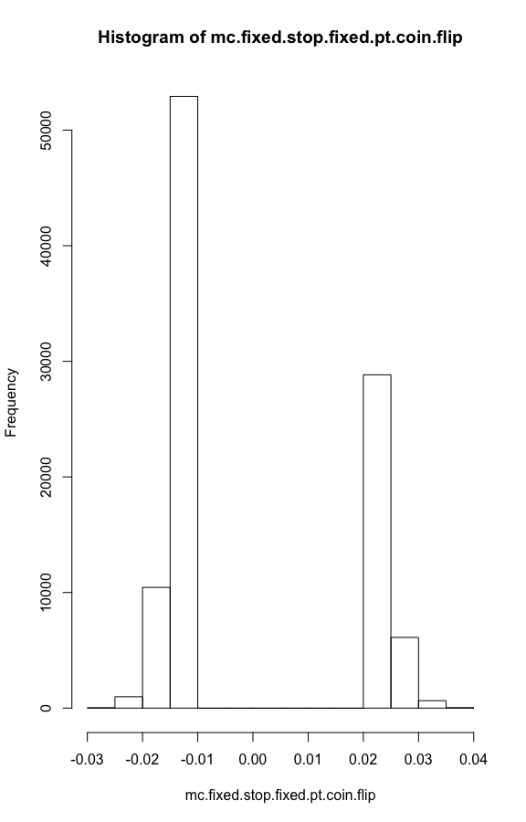
What about changing the risk to reward ratio? Say setting the stop-loss at 0.5% and really cranking the profit target up to 5%? Or taking smaller wins at the risk of larger losses - a 5% stop-loss and a 1% profit target? I won’t run it but I’ll save you the suspense; over a larger number of trades, the mean is essentially zero. *But go ahead
Test 3: Random Entry/Trailing Stop (%) Exit for Coin-Flip Stock
What about using a percent trailing stop? Does that improve returns? It seems intuitive that a trailing-stop(%) would be profitable (“you lose at most 1% AND your upside is unlimited!”). But does this apply in a random market?
Like the profit-target and stop-loss function, I am going to use the trailing stop function from the Systematic Investor Toolbox
# ----- trailing stop: exit trade once price falls below % from max price since start of trade
fn.trailing.stop.long <- function(weight = 1, price, tstart, tend, positive.percent.stop) {
    index = tstart : tend
    if(weight > 0)
        price[ index ] < (1 - positive.percent.stop) * cummax(price[ index ])
    else
        price[ index ] > (1 + positive.percent.stop) * cummin(price[ index ])
}
The trailing stop function acts to track the cumulative max over the given number of periods (for my purposes, it will be the p.periods argument from the fn.coin.flip() function). It compares the cumulative max to the change in the current price. If the percent change of the current price divided by the cumulative max is less than the positive.percent.stop then it returns FALSE. If the percent change of the current price divided by the cumulative max is more than the positive.percent.stop then it returns TRUE.
The “random entry” is the first value calculated by our fn.coin.flip() function.
The “trailing stop (%)” is then the first value of the index of returns that satisfies the fn.trailing.stop.long function. Since the fn.trailing.stop.long was created to accept a vector of stock prices, you can use the cumprod() function combined with any starting stock value as the index of stock prices to look at.
fn.trail.stop.coin.flip <- function(
                            start.value = 100,
                            p.periods = 200,
                            positive.percent.stop = .01,
                            p.prob = .5)
  {
  a <- fn.coin.flip(p.prob) # - vector of returns at p.prob
  b <- cumprod(c(start.value, a + 1)) # - vector of stock prices based on those returns
  c <- first(which(fn.trailing.stop.long(1, b, 1, p.periods,positive.percent.stop ))) # - find the index of the first instance where the trail stop fires
  c.1 <- ifelse(is.na(c) == TRUE, p.periods, c)
  d <- b[c.1] # - return the value of the index
  e <- d/start.value-1 # - exit minus entry
  return(e)
}
The fn.trail.stop.coin.flip() function returns the percentage return for the trade.
The results aren’t too promising with the trailing stop set at 1%. Again, the mean is near zero indicating that, on average, we don’t make a huge amount money over a large sample by “letting our profits run and cutting our losses short”.
mc.trail.stop.coin.flip <- replicate(100000,fn.trail.stop.coin.flip())
round(summary(mc.trail.stop.coin.flip),5)
# Min.  1st Qu.   Median     Mean  3rd Qu.     Max.
# -0.27392 -0.04873 -0.00243 -0.00015  0.04605  0.40692
hist(mc.trail.stop.coin.flip,breaks = 100)
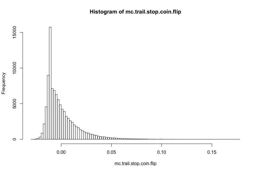
So no real difference than random entry/random exit. Maybe 1% is too tight of a stop? What about a “looser” stop of 5%?
mc.trail.stop.coin.flip.5 <- replicate(100000,fn.trail.stop.coin.flip(positive.percent.stop = .05))
round(summary(mc.trail.stop.coin.flip.5),5)

# Min.  1st Qu.   Median     Mean  3rd Qu.     Max.
# -0.27392 -0.04873 -0.00243 -0.00015  0.04605  0.40692
hist(mc.trail.stop.coin.flip.5,breaks = 100)
The 5% trailing stop didn’t really improve performance. It basically stayed the same.
Test 4: Random Entry/Trailing Stop (%) or Profit-Target(%) Exit for Coin-Flip Stock
Not to spoil the surprise, but by now you should know the result of this test before it is run. The code and results are below.
fn.trailing.stop.profit.target <- function(weight, price, tstart, tend, positive.percent.stop, p.profit) {
		index = tstart : tend
		if(weight > 0) {
			temp = price[ index ] < (1 - positive.percent.stop) * cummax(price[ index ])

			# profit target
			temp = temp | price[ index ] > (1 + p.profit) * price[ tstart ]
		} else {
			temp = price[ index ] > (1 + positive.percent.stop) * cummin(price[ index ])

			# profit target
			temp = temp | price[ index ] < (1 - p.profit) * price[ tstart ]
		}
		return( temp )
	}

fn.trail.stop.prof.targ.coin.flip <- function(
                            start.value = 100,
                            p.periods = 200,
                            positive.percent.stop = .01,
                            p.prob = .5,
                            p.profit = .02)
  {
  a <- fn.coin.flip(p.prob) # - vector of returns at p.prob
  b <- cumprod(c(start.value, a + 1)) # - vector of stock prices based on those returns
  c <- first(which(fn.trailing.stop.profit.target(1, b, 1, p.periods,positive.percent.stop, p.profit))) # - find the index of the first instance where the trail stop fires
  c.1 <- ifelse(is.na(c) == TRUE, p.periods, c)
  d <- b[c.1] # - return the value of the index
  e <- d/start.value-1 # - exit minus entry
  return(e)
}

mc.trail.stop.prof.targ.coin.flip <- replicate(100000,fn.trail.stop.prof.targ.coin.flip())
round(summary(mc.trail.stop.prof.targ.coin.flip),5)
#    Min.  1st Qu.   Median     Mean  3rd Qu.     Max.
#-0.02863 -0.01087 -0.00501 -0.00001  0.00669  0.04056
hist(mc.trail.stop.prof.targ.coin.flip,breaks = 100)
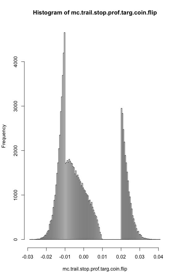
Conclusions for Coin Flip Stocks
Coin flip returns are always going to even out to zero over the long term. That is, if the market is 100% random and never trends and you have no ability to identify when the market may go up so you can enter (ie, have an edge), then there is no advantage to adding a profit-target, stop-loss or trailing-stop loss. If a market is random and you are successful with any of these implements, then it can be attributed to luck. You just happened to pick the right stretch of numbers.
But what if you can skew the coin flip in your favor - say you can guess the correct flip of the coin 53 times out of 100. What’s the effect on the coin-flip stock then?
mc.trail.stop.coin.flip.skew <- replicate(100000,fn.trail.stop.coin.flip(p.prob = .47))
round(summary(mc.trail.stop.coin.flip.skew),5)

#    Min.  1st Qu.   Median     Mean  3rd Qu.     Max.
#
-0.26530 -0.04847 -0.00219  0.00035  0.04635  0.33444
sum(unlist(mc.trail.stop.coin.flip.skew))
# [1] 34.67538
It’s a significant effect - the mean is now .03% per trade - put another way, if you traded 100,000 times, your total return would be 3467% or if you traded 100 times, you would average a total return of 3.47%. And recall that this is merely with random entries and random exits.
Having an “edge” then would seem to be important. SMB Training put it better than I could (and although the quote below name-checks trailing-stops, I would also add profit-targets and stop-losses to the statement below):
“…[T]he bottom line is if you do not have an edge in the market, you cannot make money. Period. A trailing stop is not an edge in itself (I am aware of the studies in a well-known trading book that show a profitable trading system with random entries and trailing stops. The key is that the markets tested were not random (they were real futures markets), and the exits were not random (they were a good trailing stop system). If markets were random you could not make money trading, and, if you are not convinced of that, you are missing a key piece of the intuition behind understanding price action.” Finding an edge in random markets
So if the each of the 4 random entry tests don’t add any value to a purely random stock, then the same theory should also apply to actual stock returns if the random walk theory is correct. There should be no additional return provided by adding the profit target or trailing stop. “An implication of the efficient market/random-walk theory is that no trading rule will yield an economic profit.” Testing the Random-Walk Theory. You can test this by looking at the probability distribution of the profit from a trading rule - if the random walk theory is correct, then the probability of profit should be random. Stated otherwise, you should have just “bought-and-held” because all of the entries and exits from the trading system were unecessary.
Testing on Actual Stock Data
The first step is to download historical data for the last 360 days for all of the stocks in the S&P 500. To do this, use the excellent BatchGetSymbols package. It makes quick work of downloading, organizing and saving all the data in one big data frame.
library(BatchGetSymbols)

# set dates
first.date <- Sys.Date() - 360
last.date <- Sys.Date()
freq.data <- 'daily'

# set tickers
df.SP500 <- GetSP500Stocks()
tickers <- df.SP500$Tickers

l.out <- BatchGetSymbols(tickers = tickers,
                         first.date = first.date,
                         last.date = last.date)

l.out.grouped <- l.out$df.tickers %>% group_by(ticker)
Test #1: Random Entry/Random Exit for Actual Stock Data
The function is below for entering and exiting at random.
A few key issues:
-
Since I am testing individual stocks (and not a portfolio of multiple stocks) I need to group each of the stocks individually when identifying returns. In Test #1 on actual data, I allow the individual to limit it to only entering and exiting the same ticker by setting the argument
same.ticker = TRUE. For instance, if you enter one stock long, you must sell the stock before entering another stock. Ifsame.ticker = FALSEthen the function is ignorant of which stock you enter and which stock you exit; they do not have to be the same. Note that this may provide unrealistic results as it will not exit the prior stock before entering the new one. -
There is also a maximum holding period argument. The
max.periodsargument defines the highest number of periods to hold the stock.
fn.rand.exit.actual.data <- function(data = l.out$df.tickers,
                                    max.periods = 100,
                                    same.ticker = TRUE)
                                    {
  a <- round(runif(1, min = 1, max = length(data$price.open))) # - random entry index
  b <- round(runif(1, min = a, max = length(data$price.open))) # - random exit index after entry
  c <- first(which(data$ticker[a:b] != lag(data$ticker[a:b],1))) # - where stock data changes
  d <- min(c,max.periods)
  e <- ifelse(same.ticker == TRUE,
        ifelse(data$ticker[a] == data$ticker[b], # - if ticker is the same for both
          sum(data$ret.closing.prices[a:b], na.rm = T), # - sum of all returns
          sum(data$ret.closing.prices[a:(a+d)], na.rm = T)
        ),
        sum(data$ret.closing.prices[a:b], na.rm = T)
      )
  return(e)
}

mc.rand.exit.actual.data <- replicate(100000,fn.rand.exit.actual.data())

round(summary(mc.rand.exit.actual.data),5)
#    Min.  1st Qu.   Median     Mean  3rd Qu.     Max.
#-1.64571 -0.09913  0.00626  0.01088  0.13075  1.59938

# - add in a custom function that plots a uniform distribution over the actual histogram
fn.uniform.hist <- function(data,
                    breaks, xlab = "Percent Return", main = "Frequency of Returns")
    {
  h <- hist(data, breaks = breaks, density = breaks, col = "gray", xlab = xlab, main = main)
  xfit <- seq(min(data), max(data), length = breaks)
  yfit <- dnorm(xfit, mean = mean(data), sd = sd(data))
  yfit <- yfit * diff(h$mids[1:2]) * length(data)
  lines(xfit, yfit, col = "black", lwd = 2)
}
The histogram looks fairly close to a normal distribution - except notice that the frequency is greater in the middle and at both ends (a “fat tail”). A brief scan of the research on this shows that there have been multiple 3, 4, 5 and 6 sigma events in the stock market.
Reduce the max holding period argument to 10 (and run the simulation 10k times rather than 100k times):
mc.rand.exit.actual.data.10 <- replicate(10000,fn.rand.exit.actual.data(max.periods = 10))

round(summary(mc.rand.exit.actual.data.10),5)
#     Min.  1st Qu.   Median     Mean  3rd Qu.     Max.
# -1.09355 -0.02947  0.01046  0.00505  0.05168  0.68247

fn.uniform.hist(mc.rand.exit.actual.data.10, breaks = 200, xlab = "Percent Return", main = "Frequency of Returns - Actual Data | Random Exit | Max Hold 10")
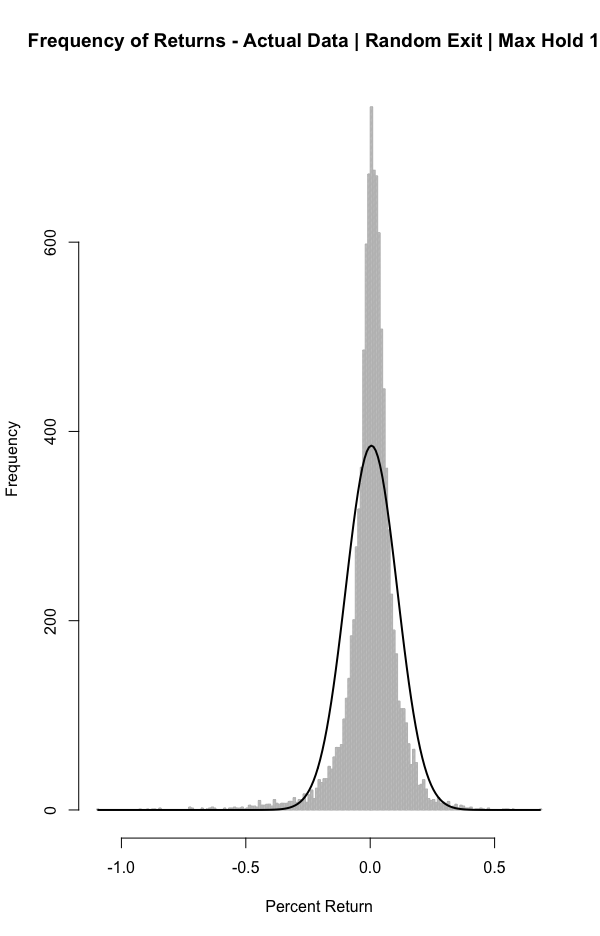
This does little to help the mean return. It actually decreased with a shorter time frame. This may lead you to explore whether longer holding times increase returns (where have I heard that before?).
Test #2: Random Entry/ Stop-Loss (%) or Profit-Target (%) Exit for Actual Stock Data
Below is the modified code for the random entry and stop-loss percentage or profit-target percentage for actual stock data.
fn.fixed.stop.fixed.pt.actual.data <- function(data = l.out$df.tickers,
                                    max.periods = 1000,
                                    same.ticker = TRUE,
                                    positive.percent.stop = .025,
                                    p.profit = .05){
  a <- round(runif(1, min = 1, max = length(data$price.open))) # - random entry index

  b <- length(data$price.open) # - end of the data vector

  c <- first(which(data$ticker[a:b] != lag(data$ticker[a:b],1))) # - where stock ticker changes as measured from the random entry

  d <- min(c,max.periods, na.rm = T) # - return length lesser of stock ticker change OR max hold periods

  a.1 <- first(which(fn.fixed.stop.fixed.pt(1, data$price.open, a, (a+d), positive.percent.stop, p.profit ))) # - return index of where stop loss or profit target fired, as measured from random entry to lesser of stock ticker change OR max hold periods

  a.2 <- min((a + a.1), min((a+d), b),na.rm = T) # - min exit index from entry (trail.stop, change of ticker, max.periods, full length of vector)

  #e <- data$price.open[[a.2]]/data$price.open[[a]]-1

  e <- sum(data$ret.closing.prices[a:a.2], na.rm = T) # - sum of all returns

  return(e)
}

# - mc analysis with max.periods at 1000, stop at 2.5% and profit target at 5%
mc.fixed.stop.fixed.pt.actual.data <- replicate(10000,fn.fixed.stop.fixed.pt.actual.data())

round(summary(mc.trail.stop.actual.data),5)

fn.uniform.hist(mc.fixed.stop.fixed.pt.actual.data, breaks = 200, xlab = "Percent Return", main = "Frequency of Returns - Actual Data | Stop Loss and Profit Target")
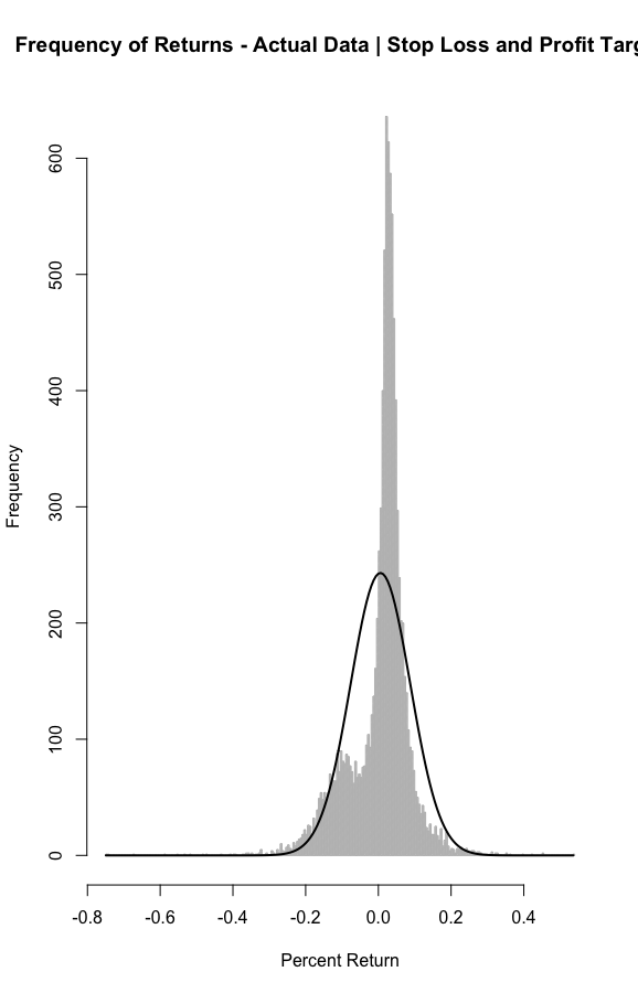
Profit target and stop loss with a 2:1 ratio didn’t return a significant non-zero mean. Again, feel free to change the parameters to see if the ultimate results stay the same.
Test #3: Random Entry/Trailing Stop Exit on Actual Stock Data
A few notes:
-
The default
max.periodsargument is now 1000 periods. The thinking is that the trailing stop should fire well before themax.periodslimit fires. -
The default
positive.percent.stopargument is now 10%.
fn.trail.stop.actual.data <- function(data = l.out$df.tickers,
                                    max.periods = 1000,
                                    same.ticker = TRUE,
                                    positive.percent.stop = .1){
  a <- round(runif(1, min = 1, max = length(data$price.open))) # - random entry index

  b <- length(data$price.open) # - end of the vector

  c <- first(which(data$ticker[a:b] != lag(data$ticker[a:b],1))) # - where stock ticker changes as measured from the random entry

  d <- min(c,max.periods, na.rm = T)

  a.1 <- first(which(fn.trailing.stop.long(1, data$price.open, a, (a+d), positive.percent.stop ))) # - find the index of the first instance where the trail stop fires a measured from rand entry to lesser of where stock ticker changes or the max hold period

  a.2 <- min((a + a.1), min((a+d), b),na.rm = T) # - min exit index (trail.stop, change of ticker, max.periods, full length)

  #e <- data$price.open[[a.2]]/data$price.open[[a]]-1

  e <- sum(data$ret.closing.prices[a:a.2], na.rm = T) # - sum of all returns

  return(e)
}

# - mc analysis 100k runs - with max.periods at 100 and positive.percent stop at 5%
# - to compare with mc.random.exit.actual.data
mc.trail.stop.actual.data.comp <- replicate(100000,fn.trail.stop.actual.data(max.periods = 100, positive.percent.stop = .05))

round(summary(mc.trail.stop.actual.data.comp),5)
#    Min.  1st Qu.   Median     Mean  3rd Qu.     Max.
#-0.90035 -0.05301 -0.01184 -0.00114  0.04277  0.88775
Comparing the trailing stop (%) exit to the purely random exit is pretty telling. Random exits net slightly more than 1% on average. Trailing stop exits (at 5%) actually lose money - to the tune of 11 bips on average. What’s more obvious is the trailing stop (%) exit has a median return of -1.18%. So, bottom line, trailing stops without an edge in the entry fair no better (and likely significantly worse) than randomly exiting the position.
Test #4: Random Entry/Trailing Stop (%) or Profit-Target (%) Exit on Actual Stock Data
The code for the random entry and trailing stop (%) or profit target (%) closely mimicks the previous code for a trailing stop. Intuitively, it seems like taking a profit at 5% and limiting loses to no more than 2.5% would be more profitable than the trailing stop (%) alone.
fn.trail.stop.profit.target.actual.data <- function(data = l.out$df.tickers,
                                    max.periods = 1000,
                                    same.ticker = TRUE,
                                    positive.percent.stop = .025,
                                    p.profit = .05){
  a <- round(runif(1, min = 1, max = length(data$price.open))) # - random entry index

  b <- length(data$price.open) # - end of the vector

  c <- first(which(data$ticker[a:b] != lag(data$ticker[a:b],1))) # - where stock ticker changes as measured from the random entry

  d <- min(c,max.periods, na.rm = T)

  a.1 <- first(which(fn.trailing.stop.profit.target(1, data$price.open, a, (a+d), positive.percent.stop, p.stop ))) # - find the index of the first instance where the trail stop fires a measured from rand entry to lesser of where stock ticker changes or the max hold period

  a.2 <- min((a + a.1), min((a+d), b),na.rm = T) # - min exit index (trail.stop, change of ticker, max.periods, full length)

  #e <- data$price.open[[a.2]]/data$price.open[[a]]-1

  e <- sum(data$ret.closing.prices[a:a.2], na.rm = T) # - sum of all returns

  return(e)
}

# - mc analysis 100k runs - with max.periods at 100, positive.percent stop at 2.5% and profit target at 5%
# - to compare with mc.random.exit.actual.data
mc.trail.stop.profit.target.actual.data <- replicate(100000,fn.trail.stop.profit.target.actual.data(max.periods = 100))

# round(summary(mc.trail.stop.profit.target.actual.data),5)
#    Min.  1st Qu.   Median     Mean  3rd Qu.     Max.
#-0.80554 -0.02529  0.00801  0.00185  0.03080  0.82386
Again, no advantage over random exits (but slightly better than trailing stop (%) alone)
What now, Donny? A Summary of Actual Data Testing
None of the exit rules got close to the mean or median return of a random exit. Disconcerting? Maybe. Or maybe it proves that you have to have an edge at entry, during the trade and at the exit. Trade management alone will not get you to the promised land.
Other Tests And Research
Momentum, Mean Reversion, Runs and Random-Walk Theory
Momentum investors believe that a positive day today will continue with a positive day tomorrow. Similarly, a negative day today will be followed by a negative day tomorrow. Put another way, the odds of an up (positive return) day following an up day are higher than a down (negative day) following an up day.
Random walk gives the odds as even that an up period will be followed by another up period. Same thing for down days; whether a down day is followed by another down day is 50% probable. (For a minute, ignore flat days to simplify the calculations). This is because a move in the future is independent of what happened in the past.
Mean reversion investments are the mirror opposite of momentum days but have the same basic premise that prior trend predicts future movement: (1) an up day means its more likely to be followed by a down day that returns to the mean, and (2) a down day is more likely to precede an up day.
Another simple statistical test is a runs test. For daily data, a run is defined as a sequence of days in which the stock price changes in the same direction. For example, consider the following combination of upward and downward price changes: + + − − + − + − − − + +. A + sign means that the stock price increased, and a − sign means that the stock price decreased. Thus the example has 7 runs, in 12 observations [note: 4 positive runs (2 of length 2 and 2 of length 1) and 3 negative runs]. Testing the Random-Walk Theory
Random walk then expects the number of runs to be n/2, where n is the number of observations.
For the 12 observations noted above, random walk predicts that, on average, there should only be 12/2 = 6 runs total in all of the observations. The standard deviation of the expected number of runs is then sqrt(n)/2 or sqrt(12)/2=1.73 runs. Assuming a normal distribution, a 2-standard-deviation confidence interval is then about 2.54 runs on the low side and 9.46 runs on the high side. A 3-standard-deviation interval (99% plus confidence) is 0.81 and 11.19, respectively.
A momentum theory or mean reversion theory is the same when looking at runs. The number of runs should be lower than what random walk expects IF we are to assume that the market trend continues (momentum) or reverts to the mean.
R provides an easy “runs”function with the rle() function. It computes the lengths and values of runs of equal values in a vector.
# - set values for an up day equal to 1, down day to -1 and a flat day to 0
a <- ifelse(l.out$df.tickers$ret.closing.prices > 0, 1, ifelse(l.out$df.tickers$ret.closing.prices < 0, -1, 0))

# - replace all NA values with 0
a[is.na(a)] <- 0

# - count the streaks of up days, down days and zero days for all of the data
b <- rle(a)

# - return a summary of the runs of up days
summary(b$lengths[b$values == 1])
#   Min. 1st Qu.  Median    Mean 3rd Qu.    Max.
#  1.000   1.000   1.000   2.009   3.000  17.000

# - return a summary of the runs of down days
summary(b$lengths[b$values == -1])
#   Min. 1st Qu.  Median    Mean 3rd Qu.    Max.
#  1.000   1.000   1.000   1.835   2.000  12.000

# - total runs - positive
length(b$lengths[b$values == 1])
# [1] 31835
length(b$lengths[b$values == -1])
# [1] 31818
On average, the data will have a run length of 2 positive days and 1.83 down days. Positive runs (ie, at least 1 up day) happened a total of 31,835 times while negative runs occured 31,818 times (note: these totals are eerily similar). Runs measurements do not measure the intensity of the streak of up or down days, only the fact that they happened a certain number of times. For example, you may have a 5 positive day run that totaled a 7% gain from start to finish and a 1 negative day run that lost 12%. Runs then don’t deal with the scale (what I like to call “intensity”) of the move.
You can compare the total number of runs for both positive and negative days.
pos.runs <- unlist(lapply(1:17, function(x)(length(b$lengths[b$values == 1 & b$lengths == x])/length(b$lengths))))

neg.runs <- unlist(lapply(1:17, function(x)(length(b$lengths[b$values == -1 & b$lengths == x])/length(b$lengths))))

tot.runs <- unlist(lapply(1:17, function(x)(length(b$lengths[b$lengths == x])/length(b$lengths))))

run.table <- cbind(
  "Run Length" = c(1:17),
  "Pos Runs - Count as % of All Runs" = round(pos.runs*100,2),
  "Neg Runs - Count as % of All Runs" = round(neg.runs*100,2),
  "Both Pos & Neg Runs - Count as % of All Runs" = round(tot.runs*100,2)
  )

library(knitr)
kable(run.table)
| Run Length | Pos Runs - Count as % of All Runs | Neg Runs - Count as % of All Runs | Both Pos & Neg Runs - Count as % of All Runs |
|---|---|---|---|
| 1 | 25.00 | 26.89 | 53.40 |
| 2 | 11.33 | 11.56 | 22.91 |
| 3 | 6.61 | 6.38 | 12.98 |
| 4 | 3.08 | 2.33 | 5.41 |
| 5 | 1.61 | 1.08 | 2.69 |
| 6 | 0.97 | 0.67 | 1.64 |
| 7 | 0.33 | 0.19 | 0.52 |
| 8 | 0.15 | 0.07 | 0.21 |
| 9 | 0.07 | 0.04 | 0.10 |
| 10 | 0.04 | 0.02 | 0.05 |
| 11 | 0.03 | 0.01 | 0.04 |
| 12 | 0.02 | 0.00 | 0.02 |
| 13 | 0.01 | 0.00 | 0.01 |
| 14 | 0.00 | 0.00 | 0.00 |
| 15 | 0.00 | 0.00 | 0.00 |
| 16 | 0.00 | 0.00 | 0.00 |
| 17 | 0.00 | 0.00 | 0.00 |
Compare the actual results to the expected results - determine if it is less than the critical value of 1.64 * sqrt(n)/2. A number of runs less than the critical value means that their is a only a 5% chance that the number of runs occurred by chance (this is roughly a 90% confidence interval).
# - find actual number of observations (removing 0 values)
n <- length(a[a != 0])

# - expected runs from random walk
exp.runs <- n/2

# - actual runs (removing 0 values)
actual.runs <- length(b$lengths[b$value != 0])

# - sd of runs and critical value
sd.exp.runs <- sqrt(n)/2
critical.value <- 1.64*sd.exp.runs

# - solve for the critical value lower limit
lower.value <- exp.runs - critical.value

> lower.value
[1] 60893.66
> actual.runs
[1] 63653
The actual number of runs is far greater than the lower value given by the 90% confidence interval. At least for this data, the number of runs is in line with what was expected by the random walk theory.
Conclusion
I can comfortably say that profitability by only managing a trade after entry is likely a losing proposition. In other words, you need to have a verifiable edge before entry to expect to make money. If nothing else, it re-inforced the rule that the market, as a whole, is likely governed by the random walk theory. Does this mean that technical analysis is always a losing proposition? I think not. The tests done above intentionally did not have a verifiable edge at entry. When a random entry/trailing stop exit strategy was employed on a stock with a skewed probability (the stock goes up 53 times out of 100), profitability was achieved. Note this was profitable even when the mean log return for the stock was set at zero.
Also - changing the mean log return to 1% and testing the coin flip stock with random entry and random exit yielded a near 0 mean return over 100k simulations. Interestingly, using the same return and a trailing stop at 10% had a .33% mean over 100k simulations. This would need additional research but it leads you to think that, possibly, the trailing stop had some value when a positive return was log normally distributed.
More research is also certainly needed on other topics. Future improvements and questions:
- How to know when you have a quantifiable edge versus a random run of favorable returns.
- Adding in account and position management rules. That is, adding in compounding to maximize geometric mean returns for each security.
- Include the Kelly Criterion and Optimal f to see if either has a meaningful effect.
- Accept the inevitable conclusion that you can’t improve performance by predicting the direction of the stock market. Past results do not predict future performance. They say luck is what happens when preparation meets opportunity. So is the key to accept that you need to stay in the game long enough to put yourself in a position to make money? Is leverage and compounding returns the best way to maximize returns (assuming a perma-bull portfolio)?
Notes and Research
- Support for the Random Walk Theory.
- Fama, Eugene F. “The behavior of stock-market prices.” The journal of Business 38.1 (1965): 34-105. PDF Link
- Fama, Eugene F. “Random walks in stock market prices.” Financial analysts journal 51.1 (1995): 75-80. PDF Link
- Pinches, George E. “The random walk hypothesis and technical analysis.” Financial Analysts Journal 26.2 (1970): 104-110. Link.
- Support for the Non-Random Walk Theory.
- Lo, Andrew W., and A. Craig MacKinlay. A non-random walk down Wall Street. Princeton University Press, 2011. PDF Link
- Hood, Donald C., Paul Andreassen, and Stanley Schachter. “II. Random and non-random walks on the New York stock exchange.” Journal of Economic Behavior & Organization 6.4 (1985): 331-338. Link
- Gup, Benton E. “A note on stock market indicators and stock prices.” Journal of Financial and Quantitative Analysis (1973): 673-682. Link
- (“STOCK MARKET PRICES DO NOT FOLLOW RANDOM WALKS: EVIDENCE FROM A SIMPLE SPECIFICATION TEST”)[https://www.nber.org/papers/w2168.pdf]
-
[PROBABILITIES AND DISTRIBUTIONS R LEARNING MODULES](https://stats.idre.ucla.edu/r/modules/probabilities-and-distributions/) - Simulating a Coin Flip in R
-
[Probabilities and Distributions R Learning Modules](https://stats.idre.ucla.edu/r/modules/probabilities-and-distributions/) - Using BatchGetSymbols to download financial data for several tickers
- SIT/bt.stop.test.r at master · systematicinvestor/SIT
- Testing the Random-Walk Theory
- Slides, Economics 466, Financial Economics
- Random Walk
- The Weakness of the Efficient-Market Theory
-
[Are Stock Returns Normally Distributed? by Tony Yiu Towards Data Science](https://towardsdatascience.com/are-stock-returns-normally-distributed-e0388d71267e) - The distribution of stock market returns - Klement on Investing.&text=As%20you%20can%20see%2C%20on,the%20normal%20distribution%20relatively%20well.)
- R Program to Generate Random Number from Standard Distributions
- 68–95–99.7 rule
- 18.05 R Tutorial: Run Length Encoding
- How do I replace NA values with zeros in an R dataframe? - Stack Overflow
- fOptions.pdf
- How To Price Stock Options Using R? - Stock Trading Ninja
- Converting Implied Volatility to Expected Daily Move - Macroption
- Black Scholes Options Pricing Model in R - Finance Train
- Trading days or calendar days for Black-Scholes parameters? - Quantitative Finance Stack Exchange
-
[The Coin Toss And Investing Success Seeking Alpha](https://seekingalpha.com/article/4138835-coin-toss-and-investing-success)