Recreating a 1976 Least Squares Betting System in R
Creating a sports betting system that beats the bookmaker is, to say the least, a challenge. In this post, I create a betting system using least squares regression that has an accuracy rate of up to 70% using out-of-sample data.
Table Contents
- Table Contents
- Research
- Testing
- Sources and Notes
Research
Implied Probability and Betting Odds - Decimal, Fraction and American Style
Implied Probability and System Value
“Implied probability is a conversion of betting odds into a percentage. It takes into account the bookmaker margin to express the expected probability of an outcome occurring….if the implied probability is less than your assessment, then it represents betting value.” See How to calculate implied probability in betting. Most betting systems seek to find value by identifying a difference between the implied probability of the bookmaker’s odds and the system’s odds. For instance, a bookmaker may be offering even (50%) odds that Team A will win versus Team B, but your system indicates Team A is a 60% favorite to win. Value then is found by betting Team A.
Converting an American Money Line to Implied Probability
A Money Line bet is a bet that a specific team will win. American based money lines can be positive or negative. Negative odds mean that the team or player is favored. Positive odds mean that the team or player is the underdog. American Money Lines are generally in multiples of $100 and indicate the amount of money you would need to risk to win the indicated amount.
| American Odds | Example | |
|---|---|---|
| Negative Money Line | Favorite | -600 = bet $600 to win $100 |
| Positive Money Line | Underdog | +450 = bet $100 to win $450 |
A negative money line means that team is favored; a line of -600 for Team A means that the bookmaker believes Team A will win 6 out of 7 times (expressed as a fraction as 1/6 or as a decimal as 1.167).
For negative American Odds, implied probability can be calculated as:
Negative American odds / (Negative American odds + 100) * 100 = Implied Probability
Note that you use the absolute value of the negative odds when solving for Implied Probability.
Conversely, a positive money line means the team is the underdog. A line of +450 (9/2 as a fraction and 5.5 as a decimal) means that Team B would only win 2 out of every 11 matches. Implied probability for positive money lines are calculated by:
100 / (positive American odds + 100) * 100 = implied probability
For our example of Team A at -600 and Team B at +450, the implied probability for each team winning is:
Team A = 600/(600+100)*100 = 85.7%

Team B = 450/(450+100)*100 = 18.1%
Bookmaker’s Margin
Note the two implied probabilities for team A and team B do not add up to 100%. This is common as bookmakers add in margin for each bet. This margin (also called “vig”) is the profit the bookmaker can expect to make assuming that there is equal action on each side of the bet. The margin can be calculated by:
Margin = (Implied Probability Team A + Implied Probability Team B)-1
So the margin for our example for Team A and Team B is:
Margin = (85.7% + 18.1%)-1 = 3.81%
Margin can also be calculated from decimal odds by:
(1/Decimal Odds option A) * 100 + (1/Decimal Odds option B) * 100 = Margin
Least Squares Regression
Basics of Least Squares Regression
Imagine that you are invited to play a round of golf with Tiger Woods. Tiger is, to say the least, a golfer that is far better than average. On the other hand, you are far below average at best and play once or twice a year. On the agreed date, it’s you and Tiger on the first tee. Tiger steps up and hammers one 350 yards down the middle. You tee up your ball, calm your nerves and whack one out there 225 yards as straight as an arrow! You repeat this feat on the 2nd and 3rd holes. Tiger even comments on how well you are playing. On the 4th hole, your confidence is high as you step up to the tee box, driver in hand. If you had to guess, where do you think your drive will end up?
If you’re like most golfers, that next shot will likely be a shank into the rough! You outpaced your ability on the first three holes. It was only a matter of time before you got back to how you really play golf - terribly! The shank off the tee is your golfing ability reverting to your average.
In statistical terms, a linear regression is based on a reversion to the mean. Just like a bad golfer shanking it off the tee after a few good shots, regression works on the theory that most things in life will return to normal.
When you hear the word regression, you probably think of how extreme performance during an earlier period most likely gets closer to average during a later period. It’s difficult to sustain an outlier performance. ThePowerRank.com.
The goal of any forecasting or predictive system is as follows:
How does a quantity in an earlier period predict the same quantity during a later period? Some quantities persist from the early to later period, which makes a prediction possible. For other quantities, measurements during the earlier period have no relationship to the later period. You might as well guess the mean, which corresponds to our intuitive idea of regression. ThePowerRank.com.
Mathematics of Least Squares Regression
Least squares regression seeks to minimize the error between a line of best fit and the measured data points on an x- and y-coordinate graph. Dependent variables are illustrated on the vertical y-axis, while independent variables are illustrated on the horizontal x-axis. In linear regression, a line of best fit is generated by using the equation of a line:
y = mx + b

Where:

- m = slope of the line
- b = y-intercept

If you square the errors and add them all together, the line with the “minimum” or least total is the line of best fit. Hence, the “least squares error.”
R Squared
Our hypothesis is that future period data can be predicted based on past period data. Later data then is dependent on our past, independent variable. The past data could be anything - margin of victory, relative strength, turnovers etc. We can then measure how well that independent data predicts future period data.
The error for each data point is the distance from the line of best fit. This error is then squared; for our purposes it doesn’t matter if the error is above or below the line. The minimum mean squared error can then be represented by the red boxes below:

How well does the red boxes explain the difference between the dependent variable and the independent variable? The difference between the expected value and the mean squared error is called variance. In simpler terms, variance measures how far the predicted values are away from the mean. The proportion of the variance that is explained by the model (the distance from the actual data point to the linear best fit line) is the measure of how well the model replicates actual data. This measure is called R-squared.
R-squared is a statistic that will give some information about the goodness of fit of a model. In regression, the R-squared coefficient of determination is a statistical measure of how well the regression predictions approximate the real data points. An R-squared of 1 indicates that the regression predictions perfectly fit the data. Coefficient of Determination on Wikipedia.
Referring to the red boxes mentioned before on ThePowerRank.com, the model represented by the best fit and the red boxes (recall they are a visual representation of the minimum mean squared error) account for 70% of the variance. In other words, the model explains 70% of the difference between the model and the actual data points. Note the original variance is illustrated by the blue boxes below and that the volume of the red boxes are 70% less than the blue boxes:

That still leaves 30% of the variance that the model does not explain. The higher the R-squared value, the better the model illustrates and predicts real world data.
Using R to Model Money Line Minimums
Remember that Money Line winners are handicapped. A heavily favored team may have a Money line of -400 which means you are laying 4 to 1 odds or betting $400 to win $100 if the team wins. Conversely, if a big underdog is listed at -600, you are getting 6 to 1 odds or betting $100 to win $600.
Many touts have systems that claim to predict the winner of a game with 70% accuracy. The system may be incredible if it hits on bets that have an implied probability of less than 70%. It’s a terrible system if you only win bets that have an implied probability greater than 70%. The real question we need to answer is whether the system will still be profitable based on different money line odds? And what are the minimum or maximum money line odds to ensure a profitable system? While it is important to have a system that has a high winning percentage, it is equally important to know the Money Line odds required to ensure you have a profitable system. Sports Betting Basics.
Modeling NFL Money Line Implied Probability Minimums
Is a system with a 40% winning percentage high enough to be profitable if the Money Line odds on all of the games it predicts average out to +125? Or is a system that picks only big favorites profitable if the average money line odds are -200?
To answer these questions, I will initially look at actual Money Line data for the National Football League (“NFL”) going back to the 2007-2008 season. Then, I will model the implied probabilities for favorites and underdogs.
Locating and Preparing the Money Line Data
Part of the challenge of any data science project is getting the data. Luckily, with enough poking around the internet, you can find just about anything. I downloaded Excel files with historical odds data from the NFL Scores and Odds Archive. These were then read into R and analyzed.
temp = list.files(pattern = "^nfl")

NFL.Odds.Data <-
    lapply(temp,function(x)(
        read_excel(x,sheet = "Sheet1")
    ))

NFL.Odds.Data <-
  rbindlist(NFL.Odds.Data)

NFL.Odds.Data$ML <- as.numeric(NFL.Odds.Data$ML)
This left me with data for approximately 9,100 teams that had money line info. I then divided the money lines between positive (underdog team) and negative (favored team). I also limited the upper and lower limits to only get Money Line information between -500 and 500.
Calculating Average Implied Probability and Expected Value for NFL Favorites and Underdogs
NFL.Odds.Data.Positive <-
  NFL.Odds.Data %>% select(ML) %>%
    group_by(ML) %>%
    filter(!is.na(ML),ML >= 10,ML <= 500)

NFL.Odds.Data.Negative <-
  NFL.Odds.Data %>% select(ML) %>%
    group_by(ML) %>%
    filter(!is.na(ML),ML >= -500,ML <= -10)
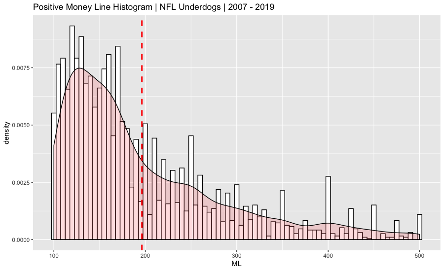
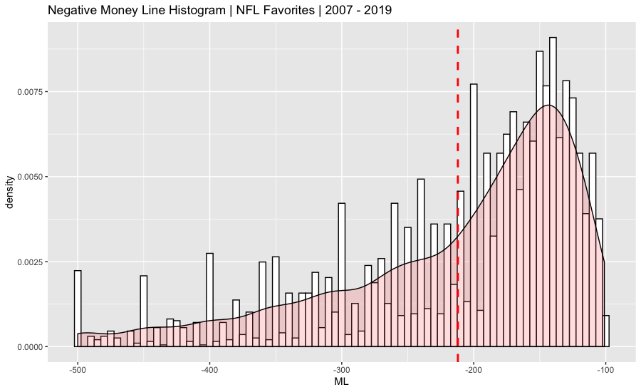
Both data sets were charted on a histogram and summarized. A probability density function was overlaid on the histogram. The vertical dashed red line on the graph represents the average.
>summary(NFL.Odds.Data$ML)
      Min.    1st Qu.     Median       Mean    3rd Qu.
-105000.00    -200.00    -110.00     -47.39     170.00
      Max.       NA's
  35000.00        770
> summary(NFL.Odds.Data.Positive$ML)
   Min. 1st Qu.  Median    Mean 3rd Qu.    Max.
  100.0   130.0   166.0   196.3   240.0   500.0
> summary(NFL.Odds.Data.Negative$ML)
   Min. 1st Qu.  Median    Mean 3rd Qu.    Max.
   -500    -260    -180    -212    -141    -101
Unsurprisingly, favorites are more expensive when compared with underdogs. On average, you would have to bet $212 on an NFL favorite to win $100, while a $100 bet on an average underdog pays out $196.
Convert American to Decimal Odds
Positive Odds (+) = (MoneyLine/100) + 1
Negative Odds (-) = (100/MoneyLine) + 1

Average Underdog MoneyLine Decimal Odds (+) = 196.3/100 + 1 = 2.963
Average Favorite MoneyLine Decimal Odds (-) = 100/212.0 + 1 = 1.471
Convert Decimal Odds to Implied Probability
Implied Probability = (1/ decimal odds) * 100

Average Underdog MoneyLine Implied Probability (+) = (1/2.963) * 100 = 33.74%
Average Favorite MoneyLine Implied Probability (-) = (1/1.471) * 100 = 67.98%
Quick summary for what the odds imply for both the favorite and the underdog:
- The odds imply a favorite wins 67.98% of the time; when this happens, you win $100 and when you lose, you lose $212.
- An underdog wins 33.7% of the time, and you win $196 when successful and lose $100 when you are not.
The implied probabilities can then be used to calculate the expected value (“EV”) for both bets. “Expected value is a predicted value of a variable, calculated as the sum of all possible values each multiplied by the probability of its occurrence.” See How to calculate expected value in betting. The Expected Value (EV) can be calculated as follows in R:
Pos.Expected.Value <-
  (NFL.Odds.Data.Positive.Implied.Prob*mean(NFL.Odds.Data.Positive$ML)) -
  ((1 - NFL.Odds.Data.Positive.Implied.Prob)* 100)

Neg.Expected.Value <-
  NFL.Odds.Data.Negative.Implied.Prob*100 -
  (1 -NFL.Odds.Data.Negative.Implied.Prob)*abs(mean(NFL.Odds.Data.Negative$ML))
This results in an EV of close to $0 for both underdogs (positive (+) money line) and favorites (negative (-) money line). This makes sense because the bookmaker’s goal is to have balanced action on both sides - equal money on favorites and underdogs. Theoretically then, based only on the implied probabilities, betting on just the favorites or just the underdogs should not give you a profitable system.
But do the actual results support the expected results? Since the odds imply a certain winning percentage, does the historical data match? Turns out, favorites win 13% less than the odds imply and underdogs win about 9% more than the odds imply.
| Implied Probability | Actual Results | Diff | |
|---|---|---|---|
| Underdog | 33.74% | 36.82% | +3.08% |
| Favorites | 67.98% | 59.89% | -8.09% |
The actual results support the conclusion that oddsmakers likely bias their lines against favorites because the betting public bet favorites a lot more than underdogs.
In 2004, University of Chicago economist Steven Levitt identified the fact that point spreads aren’t set like typical market prices, by equating relative levels of supply and demand. Instead, bookmakers set the margin to make the chance of the favorite covering the spread to be roughly 50 percent. Levitt speculated that bookmakers substantially improve their profits by biasing the spread very slightly against the favorite. This approach is profitable for bookmakers in part because, despite facing virtually even odds, people are much more likely to bet on the favorite than the underdog. See Why People Bet on the Favorite Even When the Spread Favors the Underdog on FiveThirtyEight.
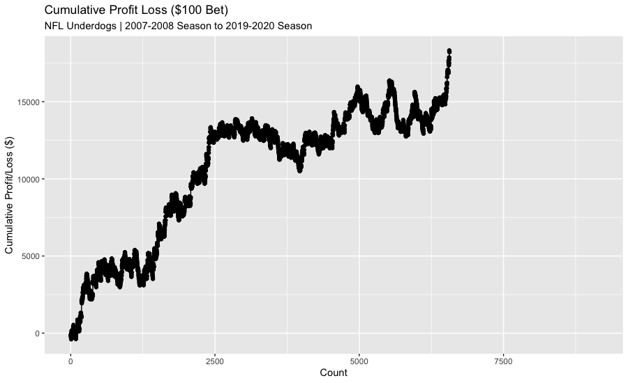
The actual results show that betting $100 on all the underdogs would be a profitable approach:
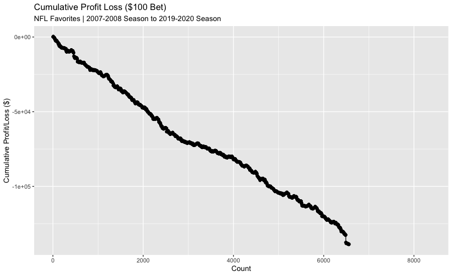
The actual results for favorites is not so great - betting $100 game results in a substantial loss!
Solving for the Required System Winning Percentage based on the Implied Money Line Odds
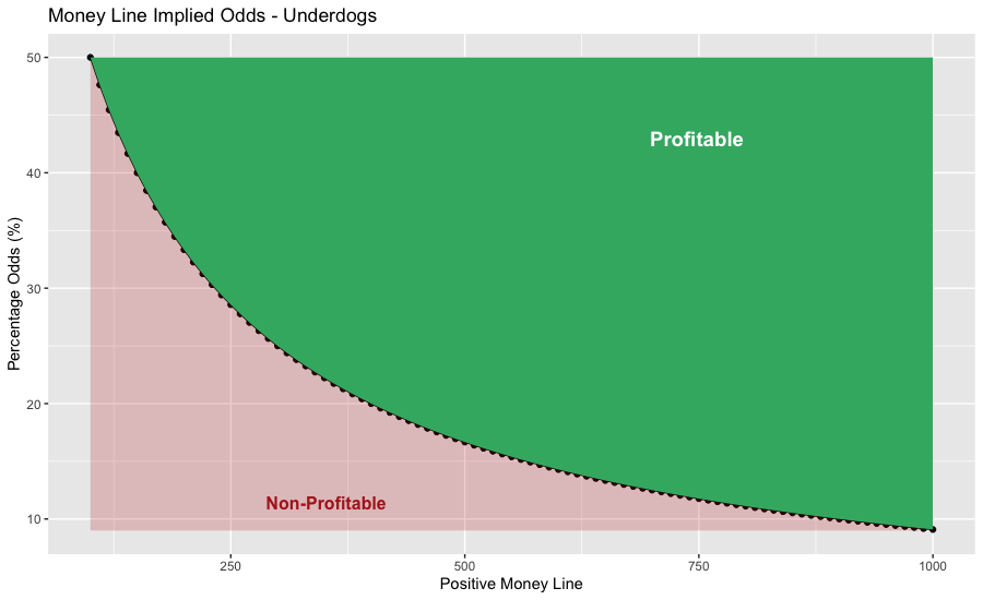
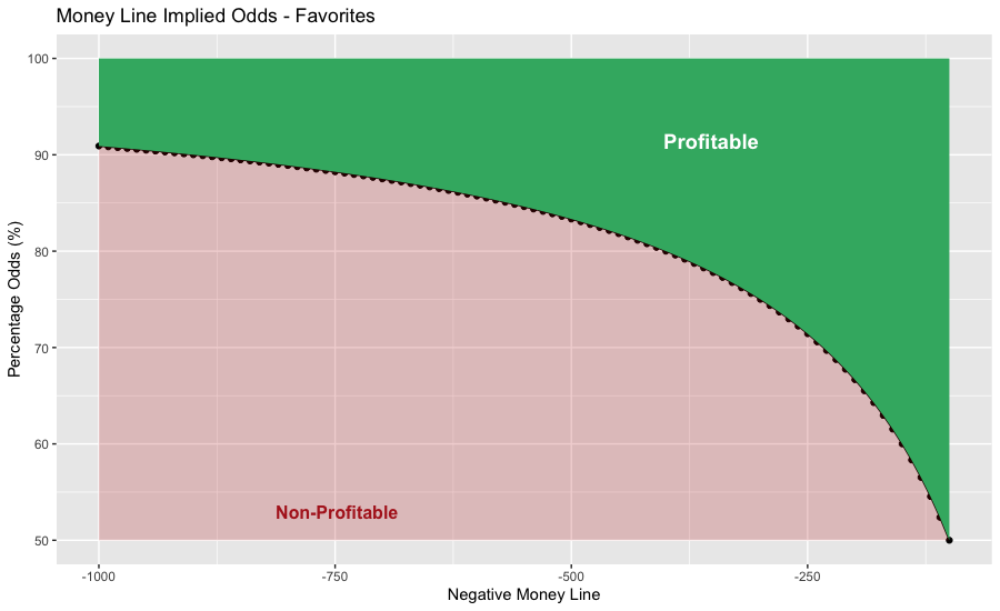
Implied probabilities can then be modeled for all money lines. Think of the implied probability as the minimum winning percentage for your betting system to be profitable. For instance, if your system only bet on favorites at -200 to win, then you would be required to win more than 66.67% to be profitable.
The charts below show the minimum system probability percentage that you would need to be profitable. Anything below the black line highlighted in red is non-profitable. Anything above the line highlighted in green is profitable.
Testing
An Overview of the 1976 System
The rating described in the 1976 paper (the “1976 System”) referenced in the title of this post relates previous outcomes to team ratings. Ratings seek to analyze the results of the competition and provide an objective measure of a team’s capabilities. Sports Ratings System on Wikipedia. In brief, the 1976 System’s team rating is defined as the average opponent rating plus the team’s average win margin. More specifically, the ratings are found as the team’s average win margin plus the 1/(n(i)+1) times the sum of each opponents average win margin. I will attempt to recreate this system using different packages within R.
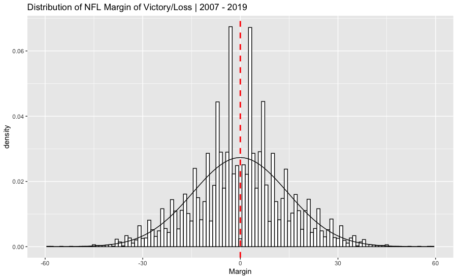
Before we create our system, let’s chart the margin of victory distribution for our historical NFL data (note: margin of victory can be positive or negative - the winner is positive and the loser is negative). It look’s roughly normally distributed. The black curve in the chart below is a plot of the normal distribution, the bars are the actual margin of victory and the red is the average (which is zero).
The main assumption that forms the basis of the least square rating system is that the difference in scores between the winning team and the losing team is directly proportional to the difference in the ratings of the two teams. Therefore, the least squares rating system attempts to express the margin of victory as a linear function of the strengths of the playing teams. Sports Ratings.
In other words, margin of victory in past periods should predict margin of victory (and therefore a win or a loss) in future periods.
The compres and comperank Packages
To help organize and sort the game data, I will use two R packages: (1) comperes which is an R tool to store and manage competition results, and (2) the companion package to compres, comperank which ranks and rates the data provided.
Data Preparation: In-Sample and Out-Of Sample Division
First, divide the data into an in-sample and out-of-sample portions with an 80%/20% ratio of in-sample to out-of-sample. Next, use the compres package to create a tibble of head-to-head matchups with the mean score difference, cumulative score difference and number of wins columns. Then, remove all of the head-to-head matchups between a team (and itself).
q <- NFL.Odds.Data %>% select(Rot,Team,Final)
names(q) <- (c("game","player","score"))
q1 <- rep(1:(length(q$game)/2),each = 2)
q$game <- q1
q <- q %>% filter(!is.na(score))
q.in.sample <- q %>% subset(game <= length(q$game)/2*.8)
q.out.sample <- q %>% subset(game > length(q$game)/2*.2)
q3 <- q.in.sample %>% h2h_long(!!! h2h_funs)
q3 <- q3 %>% filter(!is.na(num_wins),!is.na(mean_score_diff),player1 != player2)
Simple Linear Regression
The correlation matrix for the data is as follows:
               mean_score_diff mean_score_diff_pos mean_score sum_score_diff sum_score_diff_pos sum_score num_wins num_wins2   num
mean_score_diff                1.00                0.84       0.74           0.66               0.53      0.13     0.26      0.26  0.00
mean_score_diff_pos            0.84                1.00       0.64           0.55               0.56     -0.01     0.11      0.11 -0.12
mean_score                     0.74                0.64       1.00           0.49               0.38      0.13     0.16      0.16 -0.04
sum_score_diff                 0.66                0.55       0.49           1.00               0.79      0.19     0.40      0.40  0.00
sum_score_diff_pos             0.53                0.56       0.38           0.79               1.00      0.52     0.65      0.65  0.38
sum_score                      0.13               -0.01       0.13           0.19               0.52      1.00     0.94      0.94  0.97
num_wins                       0.26                0.11       0.16           0.40               0.65      0.94     1.00      1.00  0.89
num_wins2                      0.26                0.11       0.16           0.40               0.65      0.94     1.00      1.00  0.89
num                            0.00               -0.12      -0.04           0.00               0.38      0.97     0.89      0.89  1.00
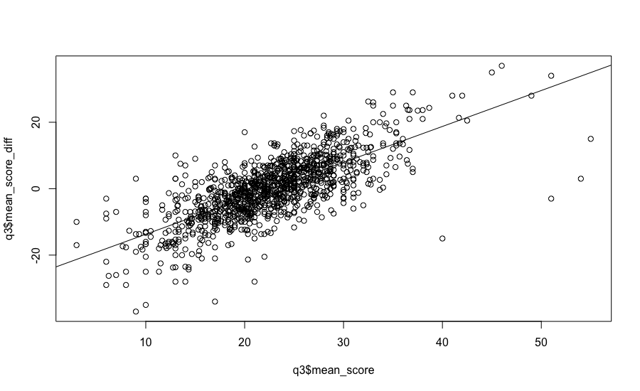
The average score difference for team 1 vs team 2 (referred to as “player 1” and “player 2” in the compres package) and the mean score of team 1 vs team 2 is positively correlated by 0.74. For simple linear regression, the format for the lm() function is “YVAR ~ XVAR” where YVAR is the dependent, or predicted, variable and XVAR is the independent, or predictor, variable. R Tutorial Series: Simple Linear Regression. The hypothesis is that the average points scored by a given team in the past can predict the margin of victory in future matchups. Our dependent or predicted y-variable then is “mean_score_diff” and our x-variable (the predictor variable) is “mean_score”.
A quick scatter plot of the in-sample data for “mean_score_diff” vs the “mean_score” shows a linear relationship between the two.
A summary of the linear regression:
Call:
lm(formula = q3$mean_score_diff ~ q3$mean_score)

Residuals:
    Min      1Q  Median      3Q     Max
-33.726  -3.755   0.236   3.734  20.483

Coefficients:
               Estimate Std. Error t value Pr(>|t|)
(Intercept)   -24.54641    0.69118  -35.51   <2e-16 ***
q3$mean_score   1.08181    0.02931   36.91   <2e-16 ***
---
Signif. codes:  0 ‘***’ 0.001 ‘**’ 0.01 ‘*’ 0.05 ‘.’ 0.1 ‘ ’ 1

Residual standard error: 6.397 on 1156 degrees of freedom
Multiple R-squared:  0.5409,	Adjusted R-squared:  0.5405
F-statistic:  1362 on 1 and 1156 DF,  p-value: < 2.2e-16
The $R^2$ value represents the proportion of variability in the response variable that is explained by the explanatory variable. For this model, 54% of the variability in score differential is explained by the historical average score of team 1 vs team 2.
Based on the regression, the difference in team 1 score vs team 2 score is equal to:
mean_score_diff = -24.56 + 1.08181 * mean_score
Using the predict() function, the mean squared error (“MSE”) for the in-sample data was 6.39 compared with an MSE of 7.53 for the out-of-sample data.
But recall - we are not concerned with win or loss margin even though the model we just created attempts to predict it. Rather, we are looking for the predicted winner of the game so that we can bet the Money Line. How often does the model predict the positive/negative margin of victory then? For the in-sample data, the model predicted the correct positive/negative margin of victory correctly 78.50% of the time. The out-of-sample data did not do as well - the model only predicted it 70.80% of the time!
But we are not concerned with the accuracy of the margin of victory OR how often it was predicted correctly. When you drill down to wins and losses, the model predicted the Money Line winner 61.89% in-sample and 61.29% out-of-sample. According to the original paper, they hit on winners in the NFL of 67.7%. Based on the large difference between the two, our model needs a little work!
Multiple Regression
One option to improve the model is to use multiple linear regression on the data. In essence, we are adding more data to help project the outcome. Our multiple linear regression model is:
fit <- lm(q3$mean_score_diff~q3$mean_score_diff_pos+q3$mean_score+q3$sum_score_diff+q3$sum_score_diff_pos+q3$sum_score+q3$num_wins)
Does the extra data lead to better accuracy when predicting postive or negative margin of victory? The $R^2$ value increased to 0.85, and the model predicted whether the whether the margin of victory would be positive or negative approximately 91% of the time for in-sample data, and 85.49% for the out-of-sample data.
The multiple regression also increased the accuracy for predicting Money Line winners (using the positive or negative approach). In-sample accuracy increased to 65.81% and (curiously) out-of-sample data accuracy improved to 70.33%.
Sources and Notes
Overview of Predictive Systems for Sports
- Least Squares Method Definition on Investopedia
- Football and Basketball Predictions Using Least Squares
- LEAST SQUARES MODEL FOR PREDICTING COLLEGE FOOTBALL SCORES
- COLLEGE FOOTBALL: A MODIFIED LEAST SQUARES APPROACH TO RATING AND PREDICTION
- How I Used Maths to Beat the Bookies
- The Problem with Win Probability - Paper from the MIT Sloan Sports Analytics Conference.
- Statistical Models Applied to the Rating of Sports Teams
- Massey’s Method
- Massey’s “Game Outcome Function”
- Prediction Tracker Archive - Football on the Prediction Tracker.
- Bibliography on College Football Ranking Systems
Odds, Implied Probability and Margin
- How to calculate implied probability in betting
- How to Calculate Betting Margin
- Trading and Betting Basics
- Information on converting Decimal, Fractional and American Odds along with a odds calculator can be found here: (1) Odds Conversion Formulas on BetSmart.co; and (2) How to Convert Betting Odds on Smarkets.com.
- For implied probability calculations, check out How to calculate implied probability in betting. You can use the implied probabilities to determine How to calculate expected value in betting.
- Historical Vegas Odds Discussion on Kaggle.
- NFL Scores and Odds Archive.
Least Squares and Regression
- Least Squares Regression on Math is Fun.
- Least Squares Method Definition on Investopedia.
- Linear Regression Overview by r-statistics.co
- Making Predictions With Simple Linear Regression Models
- Introduction to Data Science Book - 19.3 Least Squared Estimates
- The Linear Algebra View of Least-Squares Regression
- Linear Regression Example in R using lm() Function
- Ordinary Least Squares (OLS) Linear Regression in R
- A simple regression example: predicting baseball batting averages
- Linear Regression from Scratch in R
- Introduction to linear regression on RPubs.
- R Tutorial Series: Simple Linear Regression
- Data Camp Tutorial on Predict() Function
- Writing Mathematic Fomulars in Markdown
- Multiple (Linear) Regression