Machine Learning in R and Python
- [Overview](#overview)
- [Resources](#resources)
- [Saved Searches](#saved-searches)
- [Books](#books)
	- [Books - Machine Learning for Forecasting Time Series](#books-machine-learning-for-forecasting-time-series)
	- [Books - Other Types of Machine Learning](#books-other-types-of-machine-learning)
- [Articles](#articles)
	- [Basics of Machine Learning](#basics-of-machine-learning)
	- [TensorFlow](#tensorflow)
	- [Long-Short Term Memory (LSTM)](#long-short-term-memory-lstm)
		- [LSTM Basics](#lstm-basics)
		- [LSTM Code & examples](#lstm-code-examples)
		- [LSTM - Articles and Papers](#lstm-articles-and-papers)
	- [Time Series Forecasting](#time-series-forecasting)
	- [Temporal Convolutional Networks (TCN)](#temporal-convolutional-networks-tcn)
	- [Train-Test-Validation Split](#train-test-validation-split)
	- [Getting Data](#getting-data)
	- [Amazon Services (AWS)](#amazon-services-aws)
	- [Machine Learning in Sports Betting](#machine-learning-in-sports-betting)
Overview
Resources
- CRAN Task View: Machine Learning & Statistical Learning
- R Packages
- Tensorflow for R - R Studio
- Keras for R
- Cheatsheets
- Keras
Saved Searches
- “lstm time series stock market”
- “arima time series stock market”
Books
Books - Machine Learning for Forecasting Time Series
-
Hands on Machine Learning for Algorithmic Trading
- Google Books
- Summary Explore effective trading strategies in real-world markets using NumPy, spaCy, pandas, scikit-learn, and Keras
-
Machine Learning for Algorithmic Trading
- Google Books
- Summary Leverage machine learning to design and back-test automated trading strategies for real-world markets using pandas, TA-Lib, scikit-learn, LightGBM, SpaCy, Gensim, TensorFlow 2, Zipline, backtrader, Alphalens, and pyfolio.
-
Forecasting: Principles and Practice, 3rd Edition
-
Advanced Forecasting with Python
- Google Books
- Summary: Covers state-of-the-art-models including LSTMs, Facebook’s Prophet, and Amazon’s DeepAR. Includes an exhaustive overview of models relevant to forecasting. Provides intuitive explanations, mathematical background, and applied examples in Python for each of the 18 models covered
- Github Repo for Chapters from Advanced Forecasting with Python
- Hands-On Machine Learning with R
- Online Text
- Google Books
- Summary: “a practitioner’s guide to the machine learning process and a place where one can come to learn about the approach and to gain intuition about the many commonly used, modern, and powerful methods accepted in the machine learning community.”
-
Deep Learning with R, 2nd Edition
- Google Books
- Deep Learning with R introduces the world of deep learning using the powerful Keras library and its R language interface. The book builds your understanding of deep learning through intuitive explanations and practical examples.
-
Machine Learning with R: Expert Techniques for Predictive Modeling, 3rd Edition
- Hands-On Deep Learning with R
-
Hands-On Machine Learning with Scikit-Learn, Keras, and TensorFlow, 2nd Edition
Books - Other Types of Machine Learning
-
Supervised Machine Learning for Text Analysis in R
Articles
Basics of Machine Learning
TensorFlow
-
Tensor Flow Tutorial - Time Series Forecasting
-
How to Predict New Samples with Your Keras Model
-
Time Series Forecasting with TensorFlow, ARIMA, and PROPHET
Tensorflow For R
- Introduction to Tensors
- Link -
Long-Short Term Memory (LSTM)
LSTM Basics
-
Understanding LSTM Networks
-
Time Series Forecasting with the Long Short-Term Memory Network in Python
-
Multi-Step LSTM Time Series Forecasting Models for Power Usage
- Summary: In this tutorial, you will discover how to develop long short-term memory recurrent neural networks for multi-step time series forecasting of household power consumption. After completing this tutorial, you will know:
- How to develop and evaluate Univariate and multivariate Encoder-Decoder LSTMs for multi-step time series forecasting.
- How to develop and evaluate an CNN-LSTM Encoder-Decoder model for multi-step time series forecasting.
- How to develop and evaluate a ConvLSTM Encoder-Decoder model for multi-step time series forecasting.
- Link - DB
- Summary: In this tutorial, you will discover how to develop long short-term memory recurrent neural networks for multi-step time series forecasting of household power consumption. After completing this tutorial, you will know:
-
Time Series Forecasting — ARIMA, LSTM, Prophet with Python
- Summary In this article we will try to forecast a time series data basically. We’ll build three different model with Python and inspect their results. Models we will use are ARIMA (Autoregressive Integrated Moving Average), LSTM (Long Short Term Memory Neural Network) and Facebook Prophet.
- Link - DB
-
Build an LSTM Model with TensorFlow 2.0 and Keras
-
ARIMA vs Prophet vs LSTM for Time Series Prediction
LSTM Code & examples
-
LSTM in Tensorflow for Times Series forecasting
-
Time Series Forecasting using LSTM in R · Richard Wanjohi, Ph.D
-
Chapter 9 of SUpervised Machine Learning for Text Analysis in R - Long short-term memory (LSTM) networks - Supervised Machine Learning for Text Analysis in R
LSTM - Articles and Papers
-
A Comparison of ARIMA and LSTM in Forecasting Time Series
- Summary The empirical studies conducted and reported in this article show that deep learning-based algorithms such as LSTM outperform traditional-based algorithms such as ARIMA model. More specifically, the average reduction in error rates obtained by LSTM was between 84 - 87 percent when compared to ARIMA indicating the superiority of LSTM to ARIMA.
- Link - DB
-
Predictive Analytics: Time-Series Forecasting with GRU and BiLSTM in TensorFlow
-
[Paper] Deep learning based models: Basic LSTM, Bi LSTM, Stacked LSTM, CNN LSTM and Conv LSTM to forecast Agricultural commodities prices
- Summary The literature argues that an accurate price prediction of agricultural goods is a quintessence to assure a good functioning of the economy all over the world. Research reveals that studies with application of deep learning in the tasks of agricultural price forecast on short historical agricultural prices data are very scarce and insist on the use of different methods of deep learning to predict and to this reaction of filling the gap, this study employs five versions of LSTM deep learning techniques for the task of five agricultural commodities prices prediction on univariate time series dataset of Rice, Wheat, Gram, Banana, and Groundnut spanning January 2000 to July 2020.
- Link - DB
-
[Paper] Applying LSTM to time series predictable through time-window approaches.
- Summary Long Short-Term Memory (LSTM) is able to solve many time series tasks unsolvable by feed-forward networks using fixed size time windows. Here we find that LSTM’s superiority does not carry over to certain simpler time series prediction tasks solvable by time window approaches: the Mackey-Glass series and the Santa Fe FIR laser emission series (Set A). This suggests to use LSTM only when simpler traditional approaches fail.
- Link
-
[Paper] Optimizing LSTM for time series prediction in Indian stock market
- Summary Long Short Term Memory (LSTM) is among the most popular deep learning models used today. It is also being applied to time series prediction which is a particularly hard problem to solve due to the presence of long term trend, seasonal and cyclical fluctuations and random noise. The performance of LSTM is highly dependent on choice of several hyper-parameters which need to be chosen very carefully, in order to get good results. Being a relatively new model, there are no established guidelines for configuring LSTM. In this paper this research gap was addressed. A dataset was created from the Indian stock market and an LSTM model was developed for it. It was then optimized by comparing stateless and stateful models and by tuning for the number of hidden layers.
- Link - DB
Time Series Forecasting
-
Three Part Series on Time Series Analysis
-
Univariate Time Series Analysis and Forecasting with ARIMA/SARIMA
Iterated vs Direct Time Series Forecast
-
A comparison of direct and iterated multistep AR methods for forecasting macroeconomic time series
- Link - DB
- Summary Iterated multiperiod-ahead time series forecasts are made using a one-period ahead model, iterated forward for the desired number of periods, whereas direct forecasts are made using a horizon-specific estimated model, where the dependent variable is the multiperiod ahead value being forecasted. The iterated forecasts typically outperform the direct forecasts, particularly, if the models can select long-lag specifications. The relative performance of the iterated forecasts improves with the forecast horizon.
-
4 Strategies for Multi-Step Time Series Forecasting
- Link - DB
- Summary In this post, you will discover the four main strategies for multi-step time series forecasting. After reading this post, you will know: The difference between one-step and multiple-step time series forecasts. The traditional direct and recursive strategies for multi-step forecasting. The newer direct-recursive hybrid and multiple output strategies for multi-step forecasting.
-
Recursive and direct multi-step forecasting: the best of both worlds
- Link - DB
- Summary We propose a new forecasting strategy, called rectify, that seeks to combine the best properties of both the recursive and direct forecasting strategies. We find that the rectify strategy is always better than, or at least has comparable performance to, the best of the recursive and the direct strategies.
-
Machine Learning Strategies for Time Series Forecasting
- Link - DB
- Summary This chapter presents an overview of machine learning techniques in time series forecasting by focusing on three aspects: the formalization of one-step forecasting problems as supervised learning tasks, the discussion of local learning techniques as an effective tool for dealing with temporal data and the role of the forecasting strategy when we move from one-step to multiple-step forecasting.
Temporal Convolutional Networks (TCN)
-
Forecasting Gold Prices Using Temporal Convolutional Networks
- Summary Previous attempts at gold price prediction have used a variety of econometric and machine learning techniques. In particular Long Short-Term Networks (LSTMs) and more recently an ensemble of Convolutional Neural Networks (CNNs) and LSTMs have been found to have had considerable level of success in time series prediction. In this research we have conducted a comparative analysis between ARIMA, CNN, LSTM and CNN-LSTM and a recently introduced structure known as Temporal Convolutional Networks (TCNs) on gold price data spanning 20 years. The results show how TCNs produced a RMSE of 15.26 and outperformed both CNN-LSTM and LSTM with RMSE scores of 23.53 and 27.39 respectively.
- Link - DB
Convolutional Neural Networks (CNN)
-
[Paper] CNNpred: CNN-based stock market prediction using a diverse set of variables
- Link - PDF Link - DB
- Github Repo - DB Zip Repo
- Summary An attempt to classify the next days trading as ”Up” or ”Down” for the S&P500, NASDAQ, DJI, NYSE and RUSSELL stock market indices. The first model, called 2D-CNNPred, used two dimensional inputs that feed images to the CNN containing 60 days time lags and 82 explanatory variables. The second approach known as 3D-CNNPred, adds an additional dimension of features from the five financial indexes that are being predicted. Both models use multiple convolution and pooling layers and then flatten the data, which is fed to a fully-connected layer to produce the final output.
Train-Test-Validation Split
-
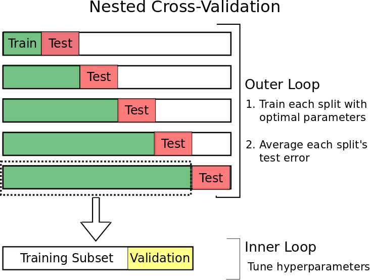
Time Series Nested Cross-Validation
- Summary This blog post discusses the pitfalls of using traditional cross-validation with time series data. Specifically, we address 1) splitting a time series without causing data leakage, 2) using nested cross-validation to obtain an unbiased estimate of error on an independent test set, and 3) cross-validation with datasets that contain multiple time series.
- Link - DB
Getting Data
-
[Colab] Introduction to Stock Analysis
-
Data Scraping in R Programming: Part 2 (Scraping HTML Data) - Analytics Steps
Amazon Services (AWS)
- Actions - Amazon Forecast
- R User Guide to Amazon SageMaker - Amazon SageMaker
- Create a Notebook Instance - Amazon SageMaker
- Time Series Forecasting Service – Amazon Forecast – Amazon Web Services
- AWS Classroom Course name: Predict the Future with Time Series Forecasting and Deep Neural Networks
- Classroom Training - Learn Cloud Skills from an Instructor - AWS
- AWS Skill Builder - Introduction to Amazon Forecast
- Time Series Forecasting Principles with Amazon Forecast - AWS Whitepaper
Machine Learning in Sports Betting
- Can We Beat the Bookmaker with Machine Learning? Predicting profitable soccer bets with a LSTM model
Building a Trading System with Machine Learning Models
Definitions
- Target variable - the variable you want to forecast
- Explanatory Variable - variable(s) that explain and forecast the target variable
- Seasonality -
- Correlation Coefficient - how much 2 variables are correlated
- Correlation Matrix - matrix that contains the correlations between each pair of variables in a dataset
- Classification - target variable is categorical (yes/no)
- Regression - supervised modeling where target variable is numeric
- Univariate Model - Only one target variable is changing over time.
- In time series analysis, the whole time series is the “variable”: a univariate time series is the series of values over time of a single quantity.
- For example, data collected from a sensor measuring the temperature of a room every second. Therefore, each second, you will only have a one-dimensional value, which is the temperature.
- Multivariate Time Series - Multiple related target variables are changing over time.
- For example, a tri-axial accelerometer. There are three accelerations, one for each axis (x,y,z) and they vary simultaneously over time.
- N Period(s) Ahead Forecast the number of time periods ahead to forecast
- Iterated forecasts multiperiod ahead time series forecasts are made using a one-period ahead model, iterated forward for the desired number of periods
- Direct Forecasts are made using a horizon-specific estimated model, where the dependent variable is the multi-period ahead value being forecasted
- Recursive forecasts are based only on values of the series up to the date on which the forecast is made. Parameters are then re-estimated in each period, for each forecasting model, using data from the beginning of the sample through the current forecasting date. Also called pseudo-out-of-sample.
Univariate Time Series Models
- Time series models are models that make a forecast of a variable by looking only at historical developments of the variable itself.
- Univariate time series models make predictions based on trends and seasonality observed in their own past and do not use explanatory variables other than the target variable: the variable that you want to forecast.
Supervised Machine Learning Models
- Model relationships between explanatory variables and a target variable
- Predictions that you would want to make may be dependent on other, independent sources of information (ie, Explanatory Variables).
- Split into: (1) classification or (2) regression
Correlations
- A correlation coefficient is always between -1 and 1.
- A positive value for the correlation coefficient means that two variables are positively correlated: if one is higher, then the other is generally also higher.
- If the correlation coefficient is negative, there is a negative correlation: if one value is higher, then the other is generally lower. This is the direction of the correlation.
- There is also a notion of the strength of the correlation.
- A correlation that is close to 1 or close to -1 is strong.
- A correlation coefficient that is close to 0 is a weak correlation.
- Strong correlations are generally more interesting, as an explanatory variable that strongly correlated to your variable can be used for forecasting it.
Types of Forecast Models
Steps to Define a Forecast Model
- Time Series: Univariate or Multivariate
- Steps Ahead: 1-step or MultiStep
- Recursiveness: Iterated or Direct
Types of Forecast Models
1. Univariate time series + 1-step ahead
- Single time series + 1 period ahead forecast
- A single time series is used to predict one single period into the future. For example, developing a model that uses the last 3 days of the local temperature at 7 a.m. to predict tomorrow’s temperature at 7 a.m.
- Example:
prediction(t+1) = model1(obs(t-1), obs(t-2), ..., obs(t-n))

# - Example training and testing data:

x_train = c(1,2,3)
y_train = c(4)

x_test = c(4,5,6)
y_test = c(7)
2. Univariate time series + Direct N-step ahead
- Single time series + Direct N-step ahead
- Single shot predictions where the entire time series is predicted at once.
- A single time series is used to create a model to predict N-periods into the future. For example, developing a model that uses the last 3 days of the local temperature at 7 a.m. to predict the temperature at 7 a.m. 3 days in the future.
- Example:
prediction(t+1) = model1(obs(t-1), obs(t-2), ..., obs(t-n))
prediction(t+2) = model2(obs(t-2), obs(t-3), ..., obs(t-n))

# - Example training and testing data:

x_train = c(1,2,3)
y_train = c(4,5,6)

x_test = c(4,5,6)
y_test = c(7,8,9)
- In the example above,
x_trainis used to predicty_trainwithout referencing what came before it. Put another way, the model doesn’t use the number4when it is predicting5and6; it only “knows” that[1,2,3]came before.
3. Univariate time series + Iterated or Recursive N-step ahead
- Single time series + Iterative N-step ahead forecast
- Autoregressive predictions where the model only makes single step predictions and its output is fed back as its input.
- Because predictions are used in place of observations, the recursive strategy allows prediction errors to accumulate such that performance can quickly degrade as the prediction time horizon increases.
- Example:
prediction(t+1) = model(obs(t-1), obs(t-2), ..., obs(t-n))
prediction(t+2) = model(prediction(t+1), obs(t-1), ..., obs(t-n))

# - Example training and testing data:

look.ahead.steps = 3

for i in 1:(look.ahead.steps){
	x_train[i] = c(1,2,3)
	y_train[i] = model %>% predict(x_train[i])
	x_train[i] = c(x_train[i], y_train[i])
}
4. Multivariate time series + 1-step Ahead
5. Multivariate time series + Direct N-step ahead
- One time series + N-step ahead
6. Multivariate time series + Iterated N-step ahead
Error and Evaluation of Models
Metric 1 - MSE
- Mean Squared Error - average of the squared errors
- Error metric –> Smaller the MSE, better the model
- Similar to variance

Metric 2 - RMSE
- Root Mean Squared Error - square root of the MSE
- Take square root –> same scale as original data
- Error metric –> Smaller the RMSE, better the model
- Similar to Standard Deviation
Metric 3 - MAE
- Mean Absolute Error - the absolute differences between the predicted and actual values per row and then average these differences.
Metric 4 - MAPE
- Mean Absolute Percent Error, is computed by taking the error for each prediction, divided by the actual value. This is done to obtain the errors relative to the actual values. This will make for an error measure as a percentage, and therefore it is standardized.
- Error Metric –> Smaller MAPE, better model
- Convert to goodness of fit by taking 1 - MAPE
Metric 5 - R-squared
- R^2 (R-squared) is a metric that is very close to the 1 – MAPE metric
- performance metric rather than an error metric
- Measured on a scale of 0 to 1 –> 0 is average
- For example, a R2 of 0.4 means it is 40% better than average
Splitting the Data
Strategy 1: Train-Test-Split
- A first split that is often deployed is the train-test split. When applying a train-test split, you split the rows of data in two. You would generally keep 20% or 30% of data in a test set.
- You can then proceed to fit models on the rest of the data: the training data.
Good v Bad Outcome - Train-Test-Split
- Good = Lower Error on training data vs test data
- Bad = Higher KPI on training data vs test data (Overfit)
- Minimum 3 observations per period
- Be aware of seasonality
Strategy 2: Train-Validation-Test Split
- Model Comparison: Benchmark performance metrics of many models
- When using the train-validation-test split, you will
- train models on the training data
- benchmark the models on the validation data, and this will be the basis for your model selection.
- use your selected model to compute an error on the test set: this should confirm the estimated error of your model.
Good v Bad Outcome - Train-Validation-Test Split
- Good = Lower Error on training data vs validation data
- Bad = Higher Error on training data vs validation data (bias in error estimate - too few points or overfit)
Strategy 3: Cross-Validation for Forecasting
K-Fold Cross-Validation
- Fit the same model k times, and you evaluate the error each time. You then obtain k error measures, of which you take the average. This is your cross-validation error.
- K - between 3 and 10
- If K = 5 then
- On those five train-test splits, you train the model on the observations that have been selected as training data
- compute the error on the observations that have been selected as the test data.
- The cross-validation error is then the average of the five test errors

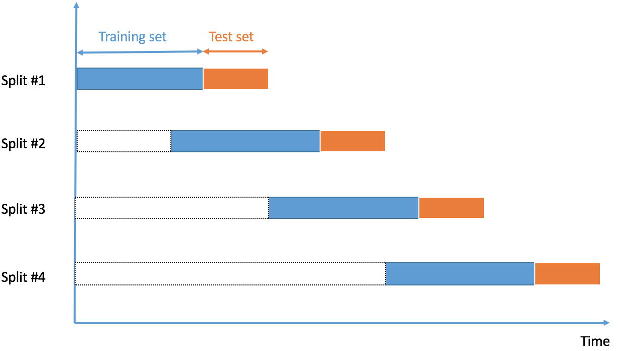
Time Series Cross-Validation
- Time series models are generally based on making forecasts based on trends and/or seasonality: they use the past of the target variable to forecast the future.
- Time Series Split: take only data that is before the test period for model training.
Rolling Time Series Cross-Validation
- Uses the same period for each fold in the cross-validation.
Backtesting
- To evaluate the performances of this strategy, you run the strategy on historical data of stock prices: what would have happened if you had sold and bought stocks at the prices you indicated. Then you evaluate how much profit you would have obtained.
- Library reco: fastquant which is available on GitHub
Safe Forecasts with a Multi-Step Strategy
- Train and tune your models using crossvalidation on the training data
- Measure predictive errors on the validation data: the model that has the best error on the validation data will be your preferred model
- Make a prediction on the test data with the selected model, and you make sure that the error is the same as the error observed on the validation data. If this is the case, you can be confident that your model should be delivering the same range of errors on future data.
- Note: you do not always have to obtain the lowest possible Mean Squared Error! Sometimes, stable performances are the most important. Other times, you may want to avoid any overestimation, while underestimations are not a problem (e.g., in a restaurant, it may be worse to buy too much food due to an overestimated demand forecast, rather than too little).
Notes & Research
General
- Mean Square Error & R2 Score Clearly Explained
- What is the difference between univariate and multivariate time series?
Training For Error Vs Profit
- backtesting - Lower MSE results in less profit when using Machine Learning - Quantitative Finance Stack Exchange - Link - DB
-
The training dilemma: loss vs profit function? by Haris (Chariton) Chalvatzis Analytics Vidhya Medium - Link - DB -
[Preparing Time Series Data for RNN in Tensorflow mobiarch](https://mobiarch.wordpress.com/2020/11/13/preparing-time-series-data-for-rnn-in-tensorflow/) - time series - LSTM Timeseries recursive prediction converge to same value - Data Science Stack Exchange
- TensorFlow for R - Introduction to Tensors
- TensorFlow for R - Working with RNNs
- RStudio AI Blog: Convolutional LSTM for spatial forecasting
-
[Time-series analysis with smoothed Convolutional Neural Network Journal of Big Data Full Text](https://journalofbigdata.springeropen.com/articles/10.1186/s40537-022-00599-y) - (PDF) LSTM Fully Convolutional Networks for Time Series Classification
- New Tab
-
[Chapter 13 Deep Learning Hands-On Machine Learning with R](https://bradleyboehmke.github.io/HOML/deep-learning.html) -
[Time Series Forecasting with Recurrent Neural Networks R-bloggers](https://www.r-bloggers.com/2017/12/time-series-forecasting-with-recurrent-neural-networks/) - RStudio AI Blog: Time Series Forecasting with Recurrent Neural Networks
-
[Learn by example RNN/LSTM/GRU time series Kaggle](https://www.kaggle.com/code/charel/learn-by-example-rnn-lstm-gru-time-series/notebook) - tensorflow - How to stack multiple lstm in keras? - Stack Overflow
-
[A Stacked GRU-RNN-Based Approach for Predicting Renewable Energy and Electricity Load for Smart Grid Operation IEEE Journals & Magazine IEEE Xplore](https://ieeexplore.ieee.org/document/9347810) - GS - ERC Credit: Todoist
- 2021 - ERC Eligibility & Credit Calculator - Gusto - Google Sheets
-
[FAQs: Employee Retention Credit under the CARES Act Internal Revenue Service](https://www.irs.gov/newsroom/faqs-employee-retention-credit-under-the-cares-act) -
[COVID-19-Related Employee Retention Credits: General Information FAQs Internal Revenue Service](https://www.irs.gov/newsroom/covid-19-related-employee-retention-credits-general-information-faqs) -
[COVID-19-Related Employee Retention Credits: Determining When an Employer’s Trade or Business Operations are Considered to be Fully or Partially Suspended Due to a Governmental Order FAQs Internal Revenue Service](https://www.irs.gov/newsroom/covid-19-related-employee-retention-credits-determining-when-an-employers-trade-or-business-operations-are-considered-to-be-fully-or-partially-suspended-due-to-a-governmental-order-faqs) -
[Employer Tax Credits Internal Revenue Service](https://www.irs.gov/coronavirus/employer-tax-credits#erclimitation) - N-2021-20
- N-2021-23
- N-2021-49
- RP-2021-33
-
[Employee Retention Credit for 2020 and 2021 Gusto](https://gusto.com/blog/taxes/employee-retention-credit) -
[Gusto Login - Payroll, Benefits, HR Gusto](https://app.gusto.com/login?ia=1&x_role_id=7757869450997147) -
[COVID-19-Related Employee Retention Credits: Determining When an Employer is Considered to have a Significant Decline in Gross Receipts and Maximum Amount of an Eligible Employer’s Employee Retention Credit FAQs Internal Revenue Service](https://www.irs.gov/newsroom/covid-19-related-employee-retention-credits-determining-when-an-employer-is-considered-to-have-a-significant-decline-in-gross-receipts-and-maximum-amount-of-an-eligible-employers-employee-retention) - There are alerts in the main content. Your session has timed out
- Inbox (462) - jake.stoetzner@gmail.com - Gmail
- booknotes-advanced-forecasting-with-python.ipynb - Colaboratory
- notes-LSTM-modeling.ipynb - Colaboratory
- doi:10.1016/j.jeconom.2005.07.020
- How To Backtest Machine Learning Models for Time Series Forecasting
- python - How can i implement multi-step forecasting for my LSTM model in keras? - Stack Overflow
- python - How to use the LSTM model for multi-step forecasting? - Stack Overflow
-
[Time Series Prediction in R Keras Kaggle](https://www.kaggle.com/code/davidchilders/time-series-prediction-in-r-keras/notebook) - TensorFlow for R – fit.keras.engine.training.model
- Time Series Forecasting with the Long Short-Term Memory Network in Python
- python - Keras LSTM - Input shape for time series prediction - Stack Overflow
- python - LSTM Nerual Network Input/Output dimensions error - Stack Overflow
- array function - RDocumentation
- Search Keras documentation
- Conv1D layer
- Crossway Storage: Rent Roll